Main / GroupTwo
Very good. The conclusions could be more eleborate (reference to theory; proposals for improvements eg. longer cables; source of potential errors, etc). rs
RADIO Assemblea Dell'Innovativa Operatori
(This is a non-Italian-speaker's attempt at a recursive acronym in Italian and it should in no way negatively reflect on Italian flair and culture! It supposedly translates to "assembly of innovative wireless operators")
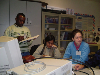
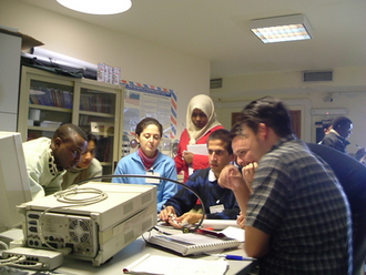
- Claro Noda, Cuba
Complexperiments - Darie Constantin Predescu, Romania
Institute for Nuclear Research - Fattaneh Mimhashemi, Iran
Ministry of Science, Research, and Technology - Fowzia Rahman, Bangladesh
Dept. of Computer Science & Engineering, Dhaka University - Jan Groenewald, South Africa
AIMS - Jose Francisco Torres, Venezuela
University of the Andes - Olusegun Aboaba, Nigeria
CURTIN - Salma Ahmed Hussein, Sudan
University of Khartoum - Walter Nakwadia Kaba, Ghana
Koffi Annan Centre of Excellence in ICT
Experiment 4: Measurement of Cable Loss with Power Meter
(from the ICTP Radio Laboratory Handbook Vol 1)
Equipment
The HP 435A power meter and the HP 8660C Synthesized Signal Generator
Procedure
- Warm up the Signal Generator and connect the power meter
- Turn RF off on the Signal Generator
- Calibrate it on 2.4 Gigahertz and 0 dBm output level
- Turn RF on
- Connect the Power Meter's power sensor and the Signal Generator with a reference cable
- Take the readings from the power meter at different frequencies for each coaxial line
Experiment 5: Measurement of Cable Loss with Spectrum Analyzer and Signal Generator
(from the ICTP Radio Laboratory Handbook Vol 1)
Equipment
The Agilent 8648C Signal Generator, and the handheld Rhodes and Schwarz FSH3, pictured below.
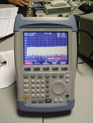
Procedure
- Warm up the Signal Generator
- Set the Signal Generator at 2.4 Gigahertz and -10 dBm output level
- Connect the reference cable between the equipment
- Calibrate for different frequencies alonog the spectrum
- Insert the coaxial lines and measure power loss at different frequencies
Experiment 6: Measurement of Cable Loss with Spectrum Analyzer and Tracking Generator
(from the ICTP Radio Laboratory Handbook Vol 1)
Equipment
The Advantest R3361A Spectrum Analyzer
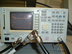
Procedure
- Warm up the spectrum analyzer
- Preset to factory defaults
- Set the frequency range to FULL RANGE
(9 kHz to 2.6 Gigahertz) - Connect the reference cable to calibrate
(Only finger-tighten the connectors) - Set the attenuation to 20 dB
(press couple / reference level) - Turn on the Tracking Generator (TG)
- Set TG to -10 dBm
- Set the Trace NORM A to ON
- Select DSP LINE
- Set the reference to -20 dBm
- Press Correct Save to offset at this level
- Insert the cable which you wish to measure
- Use Marker to aid reading attenuation along the spectrum
Results
The three experiments delivered very consistent results with similar error margings. Recommended procedure is the one employed in experiment 6, which is the simplest one.
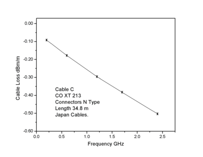
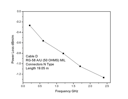
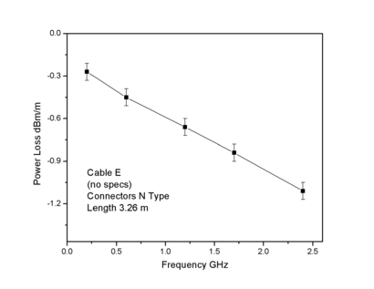
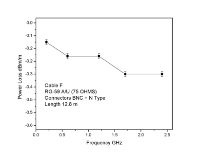
Plotting the losses at different frequencies gives a good idea of cable performance. One can see up to what frequency it's useful. Please notice that, in order to ease comparison of the graphs, the losses are given per meter length.
Graphs
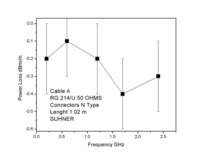
Note the error bars on cable A's graph corresponds to experiment 5, where even an excellent instrument was not able to resolve the low losses of the short cable.
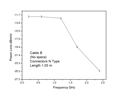
Was cable B included for illustrative purposes? Note the scale on the vertical axis is an order of magnitude larger than the other graphs.
Conclusions
Cables A and C are equivalently good cables, while cable B is pretty useless, at least for wifi applications. Cables D,E,F might be good for lab use (e.g. short distances, pigtails, and tests) but NOT for high mast antennae feeding applications.