1. Introduction to IPv6
IPv6 stands for Internet Protocol version 6, so the importance of IPv6 is implicit in its name, it’s as important as Internet! The Internet Protocol (IP from now on) was a tentative solution to data network’s needs, and has become the “de facto” standard. By now you just need to know that IP is present in all devices that are able to send and receive digital information using data networks, including the Internet. IP is standardized by the IETF, the organization in charge of all the Internet standards, what makes it easy to find, cheap, and interoperate properly between different vendor’s products and software. The fact that IP is a standard is of vital importance, because today everything is getting connected to the Internet where IP is used. All available Operating Systems and networking libraries have IP available in order to send and receive data. Included in this "everything-connected-to-Internet" is the IoT, so now you know why you are reading this chapter about IPv6, the last version of the Internet Protocol. In other words, today, the easiest way to send and receive data is using the standards used in the Internet, including the IP.
The objectives of this chapter are:
-
Briefly know about history of the Internet Protocol.
-
Know what IPv6 is used for.
-
Get the IPv6 related concepts that you will need to understand the rest of the book.
-
Give you the first practical overview of IPv6, including addresses and how an IPv6 network looks like.
1.1. A little bit of History
In the beginning of Internet, that started as a research network called ARPANET in early 1980’s,the first Internet Protocol was defined, was called IPv4 (Internet Protocol version 4). First only research centers and Universities were connected, but after the U.S. Department of Defense decided to use IP as network protocol much more funding and vendors make it to develop and be much more widely used, including vendors that implemented it. The next step was that ARPANET became Internet and get open to everybody that wanted to connect to it, including companies and public services. The exponential growth of Internet happened when HTML and web sites appeared and started to be used world-wide in the beginning of 1990’s. As a consequence there was a rapid reduction in the number of free IP addresses available under IPv4, which was never designed to scale to these levels.
In order to get more addresses, you need more bits, which means a longer IP address, which means a new architecture, which means changes to all of the routing and network software. After examining a number of proposals, the IETF settled on IPv6, recommended in January 1995 in RFC 1752, sometimes also referred to as the Next Generation Internet Protocol, or IPng. The IETF updated the IPv6 standard in 1998 with the current definition included in RFC 2460. By 2004, IPv6 was widely available from industry and supported by most new network equipment. Today IPv6 coexist with IPv4 in the Internet and the amount of IPv6 traffic is quickly growing as more and more ISPs and content providers have started to make IPv6 available.
As you can see the history of IP and Internet are almost the same, and because of this the growth of Internet has made IPv4 become insufficient for its needs, and has led to the need of a new version of IP, IPv6, that is clearly the future of Internet and the protocol to be used to interconnect devices to send and/or receive information. There are even some technologies that are being developed only with IPv6 in mind, a good example in the context of the IoT is 6LowPAN. From now on we will only center on IPv6. If you know something about IPv4, then you have half the way done, if not, don’t worry we will cover the main concepts briefly and gently.
1.2. IPv6 Concepts
We will cover the basics of IPv6, the minimum you need to know about the last version of the Internet Protocol to understand why it’s so useful for the IoT and how it’s related with other protocols like 6LowPAN covered later in this book. You need to have understood the concepts covered in the Networking Basics chapter, so you are familiar with bits, bytes, networking stack, network layer, packets, IP header, etc. You should understand that IPv6 is the equivalent to IPv4, it is a different and non-compatible protocol, with respect to IPv4. In the following figure we represent the layered model used in the Internet.
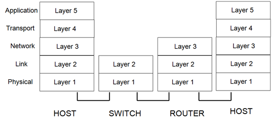
IPv6 will operate in the layer 3, also called network layer. The pieces of data handled by layer 3 are called packets. We will have hosts that could be a PC, laptop or a sensor board, sending and/or receiving data packets. Hosts will be the source or destination of the packets. Routers instead are in charge of packet forwarding, and are responsible of deciding to which other router send the packet it has received. Internet is composed of a lot of routers, interconnected between them, which receive data packets in one interface and send then as quick as possible using another interface towards another forwarding router. The first thing you have to know is how an IPv6 packet looks like:
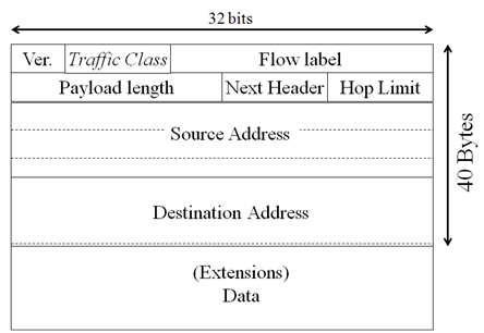
By one side you have the basic IPv6 header with a fixed size of 40 bytes, followed by upper layer data and optionally by some extensions headers, we will talk about extension headers later. As you can see there are several fields in the packet header, but compared with IPv4 header there are some improvements:
-
Number of fields have been reduced from 12 to 8 fields.
-
The basic IPv6 header has a fixed size of 40 bytes and is aligned with 64 bits, allowing a faster hardware-based packet forwarding on routers.
-
Addresses increased from 32 to 128 bits.
The most important fields are the source and destination addresses. As you already know, every IP device has a unique IP address that identifies it in the Internet. Also this IP address is used by routers to take their forwarding decisions.
IPv6 header have 128 bits for each IPv6 address, this allows for 2128 addresses (approximately 3.4×1038,i.e., 3.4 followed by 38 zeroes), compared with IPv4 that have 32 bits to encode the IPv4 address allowing for 232 addresses (4,294,967,296).
We have seen the basic IPv6 header, and we already mentioned the extensions headers. To keep the basic header simple and of a fixed size, additional features are added to IPv6 by means of extensions header.
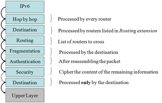
There are several extensions headers defined, as you can see in the previous figure, and they have to follow the shown order. Extensions headers:
-
Provide flexibility, for example to provide security service by ciphering the data in the packet.
-
Optimize the processing of the packet, because with the exception of the hop by hop header, they are only processed by end nodes, source and destination of the packet, not by all the routers in the path.
-
They are located as a "chain of headers" starting always in the basic IPv6 header, that use the field next header to point the first extension header.
The use of 128 bits for addresses brings some benefits:
-
Provide much more addresses, to satisfy actual and future needs, allowing for innovation.
-
Easy address auto-configuration mechanisms.
-
Easier address management/delegation.
-
Room for more levels of hierarchy and for route aggregation.
-
Ability to do end-to-end IPsec.
All IPv6 addresses could be classified into the following categories (these categories also exist for IPv4):
-
Unicast (one-to-one): used to send a packet from one source to one destination. Are the commonest ones and we will talk more about them and the sub-classes that exist.
-
Multicast (one-to-many): used to send a packet from one source to several destinations. This is possible by means of multicast routing that makes packets to replicate in some places.
-
Anycast (one-to-nearest): used to send a packet from one source the nearest destination from a set of them.
-
Reserved: Addresses or groups of them that have special use defined, for example addresses to be used on documentation and examples.
Before entering into more detail about IPv6 addresses and the types of unicast addresses, let’s see how does they look like and what are the notation rules. You need to have them clear because probably this will be the first problem you will find in practice when using IPv6, how to write an address.
Notation rules are:
-
8 Groups of 16 bits separated by “:”.
-
Hexadecimal notation of each nibble (4 bits).
-
No case sensitive.
-
Network Prefixes (group of addresses) are written Prefix / Prefix Length, i.e., prefix length indicate the number of bits of the address that are fixed.
-
Leftmost zeroes within each group could be eliminated.
-
One or more all-zero-groups could be substituted by “::”. This could be done only once.
Three first rules tell you the basis of IPv6 address notation. The first thing you should know is that hexadecimal notation is used, i.e., sixteen symbols between 0 and F. You will have eight groups of four hexadecimal symbols, each group separated by a colon ":". The last two rules are for address notation compression, we will see how they work with some examples.
Let’s see some examples:
1) If we represent all the address bits we have the preferred form, for example: 2001:0db8:4004:0010:0000:0000:6543:0ffd
2) If we use squared brackets around the address we have the literal form of the address: [2001:0db8:4004:0010:0000:0000:6543:0ffd]
3) If we apply the fourth rule, allowing compression within each group eliminating leftmost zeroes, we have: 2001:db8:4004:10:0:0:6543:ffd
4) If we apply the fifth rule, allowing compression of one or more consecutive groups of all zeroes using "::", we have: 2001:db8:4004:10::6543:ffd
Last but not least you have to understand the concept of a network prefix, that indicates some fixed bits and some non-defined bits that could be used to create new sub-prefixes or to define complete IPv6 addresses.
Let’s see some examples:
1) The network prefix 2001:db8:1::/48 (the compressed form of 2001:0db8:0001:0000:0000:0000:0000:0000) indicates that the first 48 bits will allways be the same (2001:0db8:0001) but that we can play with the other 80 bits, for example, to obtain two smaller prefixes: 2001:db8:1:a::/64 and 2001:db8:1:b::/64.
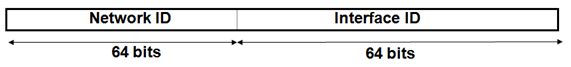
2) If we take one of the smaller prefixes defined above, 2001:db8:1:b::/64, where the first 64 bits are fixed we have the rightmost 64 bits to assign, for example, to an IPv6 interface in a host: 2001:db8:1:b:1:2:3:4. This last example allow us to introduce a basic concept in IPv6: In a LAN (Local Area Network) always a /64 prefix is used. The rightmost 64 bits, are called the interface identifier (IID) because they identify uniquely a host’s interface in the local network defined by the /64 prefix. The following figure illustrates this statement:
Now you have seen your first IPv6 addresses we can enter into more detail about two types of addresses you will find when you start working with IPv6: reserved and unicast.
The following are some reserved or special purpose addresses:
-
The unspecified address, used as a placeholder when no address is available: 0:0:0:0:0:0:0:0 (::/128)
-
The loopback address, for sending packets to itself: 0:0:0:0:0:0:0:1 (::1/128)
-
Documentation Prefix: 2001:db8::/32. This prefix is reserved to be used in examples and documentation, you have already seen it in this chapter.
The following are some types of unicast addresses:
-
Link-local: Link-local addresses are always configured in any IPv6 interface that is connected to a network. They all start with the prefix FE80::/10 and can be used to communicate with other hosts on the same local network, i.e., all hosts connected to the same switch. They couldn’t be used to communicate with other networks, i.e., to send or receive packets through a router.
-
ULA (Unique Local Address): All ULA addresses start with the prefix FC00::/7, what means in practice that you could see FC00::/8 or FD00::/8. Intended for local communications, usually inside a site, they are not expected to be routable on the Global Internet but routable inside of a more limited area such as a site.
-
Global Unicast: Equivalent to the IPv4 public addresses, are unique in the whole Internet and could be used to send a packet from anywhere in the Internet to any destination in Internet as well.
1.3. What is IPv6 used for
As we have seen IPv6 has some features that makes it easier different things like global addressing and hosts address autoconfiguration. Because IPv6 provides as much addresses as we may need for some hundreds of years, we can put a global unicast IPv6 address on almost anything we may think of. This brings back the initial Internet paradigm that every IP device could communicate with every IP device. This end-to-end communication allow for bidirectional communication all over the Internet and between any IP device, what could result in collaborative applications and new ways of storing, sending and accessing the information. In the context of this book we can, for example, think on IPv6 sensors all around the world collecting, sending and being accessed from different places to create a world-wide mesh of physical values measured, stored and processed.
The availability of a huge amount of addresses have allowed a new mechanism called stateless address autoconfiguration (SLAAC) that didn’t exist with IPv4. Following is a brief summary of the ways you can configure an address on an IPv6 interface:
-
Statically: You can decide which address you will give to your IP device and then manually configure it into the device using any kind of interface: web, command line, etc. Commonly you also have to configure other network parameters like the gateway to use to send packets out of your network.
-
DHCPv6 (Dynamic Host Configuration Protocol for IPv6): This mechanism already existed for IPv4 and the idea is the same. You need to configure a dedicated server that after a brief negotiation with the IP device assigns an IP address to it. DHCPv6 allows IP devices to be configured automatically, this is why you could find it named stateful address autoconfiguration, because the DHCPv6 server maintains an state of assigned addresses.
-
SLAAC: Stateless address autoconfiguration is a new mechanism introduced with IPv6 that allows to configure automatically all network parameters on an IP device using the router that gives connectivity to a network.
The advantage of SLAAC is that it simplifies the configuration of "dumb" devices, like sensors, cameras or any other device with low processing power. You don’t need to use any interface in the IP device to configure anything, just "plug and net". It also simplifies the network infrastructure needed to build a basic IPv6 network, because you don’t need additional device/server, you use the same router you need to send packets outside your network to configure the IP devices. We are not going to enter into details, but you just need to know that in a local network, usually called a LAN (Local Area Network), that is connected to a router, this router is in charge of sending all the information needed to the hosts using a RA (Router Advertisement) message. The router will send RAs periodically, but in order to make things happen quicker hosts can send a RS (Router Solicitation) message when its interface gets connected to the network. The router will send a RA immediately in response to the RS. The following figure show the packet exchange between a host that is just connected to a local network and some IPv6 destination in Internet:
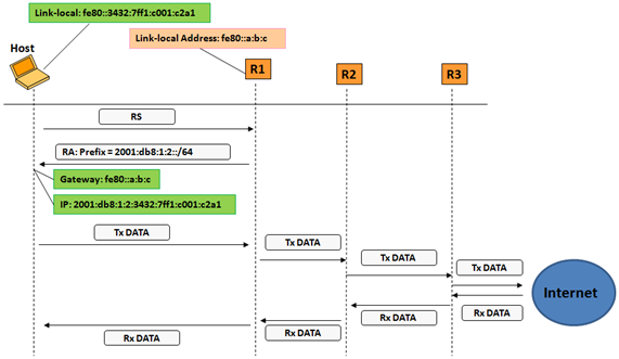
1) R1 is the router that gives connectivity to host’s network nad is sending RAs periodically.
2) Both R1 and Host have a link-local address in their interfaces connected to the host’s LAN, this address is configured automatically when the interface is ready. Our host creates it’s link-local address by combining 64 leftmost bits of the link-local’s prefix (fe80::/64) and the rightmost 64 bits of a locally generated IID (:3432:7ff1:c001:c2a1). These link-local addresses could be used in the LAN to exchange packets, but not to send packets outside the LAN.
3) The hosts needs to basic things to be able to send packets to other networks: a global IPv6 address and the address of a gateway, i.e., a router to which send the packets it wants to get routed outside its network.
4) Although R1 is sending RAs periodically (usually each several seconds) when the host get connected and has configured its link-local address, it sends a RS to which R1 responds immediately with a RA containing two things: 4.1) A global prefix of length 64 that is intended for SLAAC. The host takes the received prefix and add to it a locally generated IID, usually the same as the one used for link-local address. This way a global IPv6 address is configured in the host and now can communicate with the IPv6 Internet 4.2) Implicitly included is the link-local address of R1, because is the source address of the RA. Our host could use this address to configure the default gateway, the place to which send the packets by default, for example, to reach an IPv6 host somewhere in Internet.
5) Once both the gateway and global IPv6 address are configured, the host can receive or send information. In the figure it has something to send (Tx Data) to a host in Internet, so it creates an IPv6 packet with IPv6 destination address the one of the destination host and source address it’s recently autoconfigured global address, and sends it to its gateway, R1’s link-local address. The destination host could answer with some data (Rx Data).
1.4. Network Example
Following we will show how a simple IPv6 network will look like, including IPv6 addresses for all the networking devices.
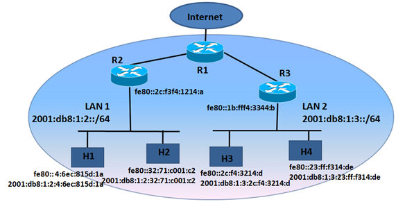
We have four hosts, or sensors, or whatever IP device you have, and we want to put two of them in two different places, for example two floors in a building. We have just put four IP devices but you can have up to 264 (18,446,744,073,709,551,616) devices connected on the same LAN.
We create two LANs with a router on each one, both routers connected to a central router (R1) that provides connectivity to Internet. LAN1 is served by R2 (with link-local address fe80::2c:f3f4:1214:a on that LAN) and uses the prefix 2001:db8:1:2::/64 announced by SLAAC. LAN2 is served by R3 (with link-local address fe80::1b:fff4:3344:b on that LAN) and uses the prefix 2001:db8:1:3::/64 announced by SLAAC.
All hosts have both a link-local IPv6 address and a global IPv6 address autoconfigured using the announced prefix by the corresponding router by means of RAs. In addition, remember that each host also configure the gateway using the link-local address used by the router for the RA. Link-local address could be used for communication between hosts inside a LAN, but for communicating with hosts in other LAN or any other network outside its own LAN a global IPv6 address is needed.
2. Short introduction to Contiki
How to install (orientative, everything should be pre-installed)
-
Know the Z1 mote: identify sensors, connectors, antenna.
-
Check the installation: toolchain location, hello world example
My first application: hello world with LEDs
-
Use the LEDs and printf to debug, use printf arguments.
-
Change timer values, triggers.
Adding sensors: analogue and digitals
-
Difference between both, basics.
-
How to connect and read: ADC, I2C
-
How to debug: enable modules printf macro, logic analyser (quick show, no hands-on for this)
3. How to install
3.1. Install VMWare for your platform
On Win and Linux: https://my.vmware.com/web/vmware/free#desktop_end_user_computing/vmware_player/6_0
On OSX you can download VMWare Fusion: http://www.vmware.com/products/fusion
3.2. Download Instant Contiki:
Instant Contiki is an entire Contiki development environment in a single download. It is an Ubuntu Linux virtual machine that runs in VMWare player and has Contiki and all the development tools, compilers, and simulators used in Contiki development installed. http://www.contiki-os.org/start.html
3.3. Start Instant Contiki
In VM, use 32 bit version, Instant_Contiki_Ubuntu_12.04_32-bit.vmdk Start Instant Contiki by running InstantContiki2.7.vmx. Wait for the virtual Ubuntu Linux boot up. Log into Instant Contiki. The password and user name is user. Don’t upgrade right now.
3.4. Update Contiki
Git is a free and open source distributed version control system designed to handle everything from small to very large projects with speed and efficiency. The main difference with previous change control tools like Subversion, is the possibility to work locally as your local copy is a repository, and you can commit to it and get all benefits of source control. Making branches and merging between branches is really easy.
To learn more about GIT there are some great tutorials online:
A nice graphical introduction to Git is available here: http://rogerdudler.github.io/git-guide/

GitHub is a GIT repository web-based hosting service, which offers all of the distributed revision control and source code management (SCM) functionality of Git as well as adding its own features. Unlike Git, which is strictly a command-line tool, GitHub provides a web-based graphical interface and desktop as well as mobile integration. It also provides access control and several collaboration features such as wikis, task management, and bug tracking and feature requests for every project.
Contiki source code is maintained and hosted at Github: https://github.com/contiki-os/contiki.
The advantage of using GIT and hosting the code at github is allowing people to fork the code, develop on its own, and then contribute back and share your progress.
To update our code to the latest available contiki code, open a terminal and write:
cd $HOME/contiki
git fetch origin master
git pull origin master
git log to see the latest log
ADD GIT FOR EXAMPLES
3.5. Check installation: toolchain location
Open a terminal and write:
msp430-gcc --versionCheck if you have version 4.7. If not, download the latest toolchain version here: http://sourceforge.net/projects/zolertia/files/Toolchain/
3.6. Check installation: examples
Open a terminal and write:
cd examples/hello-world
make TARGET=z1 savetarget
so it know that when you compile you do so for the z1 mote. You need to do this only once per application.
make hello-worldit starts compiling (ignore the warnings)
3.7. Check z1 connection to the virtual machine
Connect the mote via USB.
In VM player: Player → Removable Devices → Signal Integrated Zolertia Z1 → Connect
In VMWare Fusion: Devices → USB Devices → Silicon Labs Zolertia Z1
Open a terminal and write:
make z1-motelist
user@instant-contiki:~/contiki/examples/hello-world$ make z1-motelist
using saved target 'z1'
../../tools/z1/motelist-z1
Reference  Device       	Description
---------- ---------------- ---------------------------------------------
Z1RC0336   /dev/ttyUSB0 	Silicon Labs Zolertia Z1
Save the reference ID for next lab sessions (Z1RC0336). Each mote has a unique reference number. The port name is useful for programming and debugging.
Upload the preloaded Hello World application to the Z1 mote
Open a terminal and write:
make hello-world.upload MOTES=/dev/ttyUSB0if you don’t use the MOTE part, the system will install on the first device it finds. It is OK if you only have one device.
If you get this error:
serial.serialutil.SerialException: could not open port /dev/ttyUSB0: [Errno 13] Permission denied: '/dev/ttyUSB0'you need to add yourself to the dialout group of Linux. You do it this way:
sudo usermod -a -G dialout userenter the root password, which is user
sudo rebootpassword is user.
open terminal and go again to /contiki/examples/hello-world and enter again
make hello-world.upload  MOTES=/dev/ttyUSB0
make z1-reset && make login
the first command resets the mote and the second one connects to the serial port and displays the result on the screen
Sceenshot missing
Note that the node ID is displayed.
4. My first applications
4.1. Hello world with LEDs
Let’s see the main components of the Hello World example. View the code with:
gedit hello-world.cWhen starting Contiki, you declare processes with a name. In each code you can have more processes. You declare the process like this:
PROCESS(hello_world_process, "Hello world process"); (1)
AUTOSTART_PROCESSES(&hello_world_process); (2)| 1 | hello_world_process is the name of the process and "Hello world process" is the readable name of the process when you print it to the terminal. |
| 2 | The AUTOSTART_PROCESSES(&hello_world_process); tells Contiki to start that process when it finishes booting. |
/*---------------------------------------------------------------------------*/
PROCESS(hello_world_process, "Hello world process");
AUTOSTART_PROCESSES(&hello_world_process);
/*---------------------------------------------------------------------------*/
PROCESS_THREAD(hello_world_process, ev, data) (1)
{
  PROCESS_BEGIN(); (2)
  printf("Hello, world\n"); (3)
  PROCESS_END(); (4)
}| 1 | You declare the content of the process in the process thread. You have the name of the process and callback functions (event handler and data handler). |
| 2 | Inside the thread you begin the process, |
| 3 | do what you want and |
| 4 | finally end the process. |
The next step is adding a LED and the user button. Add picture.
Let’s create a new file. Go to: /home/user/contiki/examples/z1 with
cd /home/user/contiki/examples/z1Let’s name the new file test_led.c with
gedit test_led.c.You have to add the dev/leds.h which is the library to manage the LED lights. To check the definition go to /home/user/contiki/core/dev.
Available LEDs commands:
unsigned char leds_get(void);
void leds_set(unsigned char leds);
void leds_on(unsigned char leds);
void leds_off(unsigned char leds);
void leds_toggle(unsigned char leds);
Available LEDs:
LEDS_GREEN
LEDS_RED
LEDS_BLUE
LEDS_ALL
Now try to turn ON only the red LED and see what happens
#include "contiki.h"
#include "dev/leds.h"
#include <stdio.h>
//-----------------------------------------------------------------
PROCESS(led_process, "led process");
AUTOSTART_PROCESSES(&led_process);
//-----------------------------------------------------------------
PROCESS_THREAD(led_process, ev, data)
{
  PROCESS_BEGIN();
  leds_on(LEDS_RED);
  PROCESS_END();
}
We now need to add the project to the makefile. So edit Makefile and make sure you have:
CONTIKI_PROJECT = test-phidgets blink test-adxl345 test-tmp102 test-light-ziglet test-battery test-sht11 test-relay-phidget test-tlc59116
CONTIKI_PROJECT += test_led
Now let’s compile and upload the new project with:
make clean && make test_led.upload MOTES=/dev/ttyUSB0
the make clean is used to erase previously compiled objects. Now the LED is red!
Missing pictures.
| Exercise: try to switch on the other LEDs. |
4.2. Printf
You can use prinf to visualize on the console what is happening in your application. It is really useful to debug your code, as you can print values of variables.
Let’s try to print the status of the LED, using the unsigned char leds_get(void); function that is available in the documented functions (see above).
Get the LED status and print its status on the screen.
#include "contiki.h"
#include "dev/leds.h"
#include <stdio.h>
char hello[] = "hello from the mote!";
//-----------------------------------------------------------------
PROCESS(led_process, "led process");
AUTOSTART_PROCESSES(&led_process);
//-----------------------------------------------------------------
PROCESS_THREAD(led_process, ev, data)
{
  PROCESS_BEGIN();
  leds_on(LEDS_RED);
  printf("%s\n", hello);
  printf("The LED %u is %u\n", LEDS_RED, leds_get());
  PROCESS_END();
}
If one LED is on, you will get the LED number (LEDs are numbered 1,2 and 4).
| Exercise: what happens when you turn on more than one LED? What number do you get? |
4.3. Button
We now want to detect if the user button (see picture) has been pushed.
Create a new file in /home/user/contiki/examples/z1 called test_button.c
The button in Contiki is considered as a sensor. We are going to use the dev/button-sensor.h library. It is a good process to give the process a meaningful name so it reflects what the process is about.
Here is the code to print the button status:
#include "contiki.h"
#include "dev/leds.h"
#include "dev/button-sensor.h"
#include <stdio.h>
//-----------------------------------------------------------------
PROCESS(button_process, "button process");
AUTOSTART_PROCESSES(&button_process);
//-----------------------------------------------------------------
PROCESS_THREAD(button_process, ev, data)
{
  PROCESS_BEGIN();
  SENSORS_ACTIVATE(button_sensor);
  while(1) {
  PROCESS_WAIT_EVENT_UNTIL((ev==sensors_event) && (data == &button_sensor));
  printf("I pushed the button! \n");
  }
  PROCESS_END();
}
Let’s modify the Makefile to add the new file.
CONTIKI_PROJECT += test_buttonYou can leave the previously created test_led in the makefile. This process has an infinite loop (given by the wait()) to wait for the button the be pressed. The two conditions have to be met (event from a sensor and that event is the button being pressed) As soon as you press the button, you get the string printed.
| Exercise: switch on the LED when the button is pressed. Switch off the LED when the button is pressed again. |
4.4. Timers
Create a new file in /home/user/contiki/examples/z1 called test_timer.c.
You don’t need any new library as the timer is part of Contiki’s core.
We create a timer structure and we set the timer to expire after a given number of seconds. Then when the timer is expired we execute the code and restart the timer. This is the basic type of timer. Contiki has three types of timers.
#include "contiki.h"
#include "dev/leds.h"
#include "dev/button-sensor.h"
#include <stdio.h>
#define SECONDS 2
//-----------------------------------------------------------------
PROCESS(hello_timer_process, "hello world with timer example");
AUTOSTART_PROCESSES(&hello_timer_process);
//-----------------------------------------------------------------
PROCESS_THREAD(hello_timer_process, ev, data)
{
  PROCESS_BEGIN();
  static struct etimer et;
  while(1) {
  etimer_set(&et, CLOCK_SECOND*SECONDS); (1)
  PROCESS_WAIT_EVENT(); (2)
  if(etimer_expired(&et)) {
    printf("Hello world!\n");
    etimer_reset(&et);
  }
  }
  PROCESS_END();
}| 1 | CLOCK_SECOND is a variable that relates to the microcontroller ticks. As Contiki runs on different platforms, the value of CLOCK_SECOND is different in different devices. This is related to the frequency of the processor. In Z1 it is 128. |
| 2 | PROCESS_WAIT_EVENT(); waits for any event to happen. |
| Excercise: can you print the value of CLOCK_SECOND to count how many ticks you have in one second? Try to blink the LED for a certain number of seconds. A new application that starts only when the button is pressed and when the button is pressed again it stops. |
5. Sensors
The Z1 has two built in digital sensors: temperature and 3 axis acceleration. The main difference between analog and digital sensors are the power consumption (lower in digital) and the protocol they use. Analog sensors require being connected to ADC (analog to digital converters) which translate the analog (continuous) reading to a digital value (in millivolts). The quality and resolution of the measure depends on both the ADC (resolution is 12 bits in the Z1) and on the sampling frequency. As a rule of thumb, you need to have double sampling frequency as the phenomena you are measuring. As an example, if you want to sample human sound (8 kHz) you need to sample at twice that frequency (16 kHz minimum).
5.1. Analog Sensors
There is one analog sensor in the Z1, and it provides the battery level expressed in milliVolts. There is an example in the Contiki example folder called test-battery.c. The example includes the battery level driver (battery-sensor.h). It activates the sensor and prints as fast as possible (with no delay) the battery level. When working with the ADC you need to convert the ADC integers in milliVolts. This is done with the following formula:
float mv = (bateria * 2.500 * 2) / 4096;
We are powering the Z1 with 5 Volts (this is why we multiply by 5). We divide the raw value by 4096 as it is a 1 shifted to 12 positions on the left (as the precision of the ADC is 12 bits). The internal power of the Z1 is 3V. There is an internal voltage divider that converts from 5V to 3.3V. If you connect the Z1 to the USB port, you will always get the highest value (around 3V). Two value are printed by the code in two columns: the raw value from the ADC and the converted value in milliVolts.
5.2. External analog sensor:
We can connect an external analog sensor. As an example, let’s connect the precision light sensor. It is important to know the voltage required by each sensor. If the sensor can be powered at 3V, it should be connected to the phidgets connector in the top row. If the sensor is powered at 5V it can be safely connected to the phidgets bottom row. Only if the mote is powered by USB, then you can use the 5V sensor. Insert phidgets Insert picture. If you use the phidgets cable, there is a single way to connect the node. Insert datasheet of the light sensors.
You need to convert the values coming from a 5V sensors as there is an internal voltage divider.
There is an example called test-phidgets.c. This will read values from an analog sensor and print them to the terminal. Connect the light sensor to the 3 V phidget connector.
As this is an official example, there is no need to add it to the Makefile (it is already there!).
Let’s compile the example code:
make clean && make test-phidgets.upload MOTES=/dev/ttyUSB0and connect to the node:
make z1-reset && make loginThis is the result:
Starting 'Test Button & Phidgets'
Please press the User Button
Phidget 5V 1:123
Phidget 5V 2:301
Phidget 3V 1:1710
Phidget 3V 2:2202
The light sensor is connected to Phidget 3V 2, so the raw value is 2202. Try to illuminate the sensor with a flashlight (from your mobile phone, for example) and then to keep it in your hand so that no light can reach it. http://www.phidgets.com/products.php?product_id=1127_0
Sensor Properties Sensor Type Light Sensor Output Type Non-Ratiometric Response Time Max 20 ms Measurement Error Max ± 5 % Peak Sensitivity Wavelength 580 nm Light Level Min 1 lx Light Level Max (3.3V) 660 lx Light Level Max (5V) 1 klx
As you can see, the light sensor can be connected to both the 5 V and 3.3 V phidget connector. The max measurable value changes depending where you connect it. The formula to translate SensorValue into luminosity is: Luminosity(lux)=SensorValue
| Exercise: make the sensor take sensor readings as fast as possible. Print on the screen the ADC raw values and the millivolts (as this sensor is linear, the voltage corresponds to the luxes). What are the max and min values you can get? What is the average light value of the room? Create an application that turns the red LED on when it is dark. When it is light, turn the green LED on. In between, switch off all the LEDs. Add a timer and measure the light every 10 seconds. |
5.3. Internal digital sensor
The Z1 has an internal digital sensor: the 3 axis accelerometer. There is an example called test-adxl345.c. You don’t need to add it to the Makefile. Once uploaded, this is the result:
~~[37] DoubleTap detected! (0xE3) -- DoubleTap Tap
x: -1 y: 12 z: 223
~~[38] Tap detected! (0xC3) -- Tap
x: -2 y: 8 z: 220
x: 2 y: 4 z: 221
x: 3 y: 5 z: 221
x: 4 y: 5 z: 222
The accelerometer can give data in x,y and z axis and has three types of interrupts: when you do a single tap, when you do a double tap and when you let the sensor free-fall (pay attention not to damage the mote!). Try tapping once and twice. The code has two threads, one for the interruptions and the other for the LEDs. When Contiki starts, it triggers both the processes. The led_process thread triggers a timer that waits before turning off the LEDs. This is mostly done to filter the rapid signal coming from the accelerometer. The other process is the acceleration one. It assigns the callback for the led_off event. Interrupts can happen at any given time, are non periodic and totally asynchronous. They can be triggered by external sources (sensors, interrupt pins, etc) and should be cleared as soon as possible. When an interrupts happens, the interrupt handler (which is a process that checks the interrupt registers to find out which is the interrupt source) manages it and forwards it to the subscribed callback. In this example, I first start the accelerometer and then map the interrupts from the accelerometer to a specific callback function. Interrupt source 1 is mapped to the free fall callback handler and the tap interrupts are mapped to the interrupt source 2.
  /* Start and setup the accelerometer with default values, eg no interrupts enabled. */
  accm_init();
  /* Register the callback functions for each interrupt */
  ACCM_REGISTER_INT1_CB(accm_ff_cb);
  ACCM_REGISTER_INT2_CB(accm_tap_cb);
  /* Set what strikes the corresponding interrupts. Several interrupts per pin is
    possible. For the eight possible interrupts, see adxl345.h and adxl345 datasheet. */
We then need to enable the interrupts like this:
accm_set_irq(ADXL345_INT_FREEFALL, ADXL345_INT_TAP + ADXL345_INT_DOUBLETAP);
What happens in the while cycle is that we read the values from each axis every second. If there are no interrupts, this will be the only thing shown in the terminal.
| Exercise: put the mote in different positions and check the values of the accelerometer. Try to understand what is x, y and z. Measure the max acceleration by shaking the mote. Turn on and off the LED according to the acceleration on one axis. Image with axis |
5.4. External digital sensor
The ZIG001-mini is a digital temperature sensor.
The advantage of using digital sensors is that you don’t have to do calibration of your own as they come factory-calibrated. They usually have a low power current consumption compared to their analog peers. They allow a more extended set of commands (turn on, turn off, configure interrupts). If you have a digital light sensor, you can set a threshold value when the sensor sends an interrupt, without the need for continuous polling.
The example is available as test-sht11.c. The light digital sensor is also given as example in the same folder.
Temperature:   27 degrees Celsius
Rel. humidity: 67%
Temperature:   27 degrees Celsius
Rel. humidity: 66%
Temperature:   27 degrees Celsius
Rel. humidity: 65%| Exercise: convert the temperature to Fahrenheit. Try to get the temperature and humidity as high as possible (without damaging the mote!). Try to print only “possible” values (if you disconnect the sensor, you should not print anything, or print an error message!). |
6. Sending Data to Ubidots:
What is Ubidots Get API key and variable ID
We can send data from the sensors to Ubidots to visualize and generate events. We need two software components to send data. We will modify an existing Z1 example from today. We will send data from the temperature sensor to the serial port of the PC. The PC will then parse the data and send it to Ubidots using their API with a python script. For the data to be parsed correctly it must follow a certain format (like tab separated, comma separated or others).
In this case we will use a Contiki application that handles the serial formatting to be sent to the python script. Apps are created to provide extra features that can be used directly by other applications. Apps are placed in the apps folder of Contiki. The Makefile of an APP has the following naming convention:
Makefile.serial-shellAnd inside you must specify which are the source codes that will be used, in this case:
serial-ubidots_src = serial-ubidots.cThis is what the serial-ubidots serial will look like:
#include <string.h>
#include "serial-ubidots.h"
void
send_to_ubidots(const char *api, const char *id, uint16_t val)
{
  unsigned char buf[6];
  snprintf(buf, 6, "%d", val);
  printf("\n\r%s\t", api);
  printf("%s\t", id);
  printf("%s\n\r", buf);
}
You need to declare a header file serial-ubidots.h as well:
#define VAR_LEN 24
#define UBIDOTS_MSG_LEN (VAR_LEN + 2)
struct ubidots_msg_t {
  char var_key[VAR_LEN];
  uint8_t value[2];
};
void send_to_ubidots(const char *api, const char *id, uint16_t val);
We have also created a data structure which will simplify sending this data over a wireless link, we will talk about this a bit later.
Now that we have created this APP, we should add it to our example code (that sends temperature to Ubidots), the proper way is to edit the Makefile we have already know at examples/z1 and add serial-ubidots to the APPS argument:
APPS = serial-shell serial-ubidotsAnd now let’s edit the test-tmp102.c example to include the serial-ubidots application, first add the serial-ubidots header as follows:
#include "serial-ubidots.h"Then we should create 2 new constants with the API key and Variable ID, obtained at Ubidots site as follows:
static const char api_key[] = "fd6c3eb63433221e0a6840633edb21f9ec398d6a";
static const char var_key[] = "545a202b76254223b5ffa65f";
It is a general good practice to declare constants values with as “const”, this will save some valuable bytes for the RAM memory :) Change the polling interval to avoid flooding Ubidots and kicking us out :)
#define TMP102_READ_INTERVAL (CLOCK_SECOND * 15)Then we are ready to send our data to Ubidots, first change the call to the tmp102 sensor to have the value with 2 digits precision, and send it over to Ubidots, replace as follows:
PRINTFDEBUG("Reading Temp...\n");
raw = tmp102_read_temp_x100();
send_to_ubidots(api_key, var_key, raw);
Upload the code to the Z1:
make MOTES=/dev/ttyUSB0 test-tmp102.upload && make MOTES=/dev/ttyUSB0 z1-reset && make MOTES=/dev/ttyUSB0 login
This is what you will see on the screen:
fd6c3eb63433221e0a6840633edb21f9ec398d6a
545a202b76254223b5ffa65f    2718
Notice that you must divide by 100 to get the 27.18ºC degree value, this can be done easily on Ubidots.
Ubidots Python API Client
The Ubidots Python API Client makes calls to the Ubidots Api. The module is available on PyPI as “ubidots”. To follow this quickstart you’ll need to have python 2.7 in your machine (be it a computer or an python-capable device), which you can download at http://www.python.org/download/.
You can install pip in Linux and Mac using this command:
$ sudo easy_install pipInstalling the Python library Ubidots for python is available in PyPI and you can install it from the command line:
$ sudo pip install ubidots==1.6.1The python script on the PC is called UbidotsPython.py and is located in the tools/z1 directory. The script parses the serial data and sends it to Ubidots. to execute it, run:
user@instant-contiki:~/contiki/tools/z1$ python UbidotsPython.py -p /dev/ttyUSB0
In which -p is the argument to tell the Python script to connect to our mote at the given port.
If you connect to Ubidots, you will immediately see the values coming in.
To enable printing debug information from the Python script to the console, enable the following value at the UbidotsPython.py file:
# Enable to print extended information
DEBUG_APP = 1
The data is sent to Ubidots as long as the pyhton script is running. You can have it working in the background by adding & at the end of the script call. While the python script is running, you cannot program the node!
As the temperature sensor is located next to the USB connector, it tends to heat up. A realistic value is few degrees lower than the measured on. To get more reliable temperature measurements while connected to the USB, use an external temperature sensor!
Don’t forget that Ubidots will not accept more than one measurement every 15 seconds. If you send data more frequently, you will lose the connection.
To divide the incoming data by 100, you should name it as derived variable as follows: create a temperature variable with the raw data and then the derived variable by dividing the temperature variable by 100.
In Ubidots your data will show up as follows:
7. Wireless with Contiki:
-
Set up Node ID, MAC address, ID used by Contiki.
-
Simple application: UDP broadcast
-
Simple application: UDP Server and client
-
Check mote to mote communication
-
Check ETX, LQI, RSSI.
-
Change the Channel, PAN ID.
-
Debug: use Packet sniffer/Wireshark
-
RSSI scanner example
8. Set up Node ID, MAC address, ID used by Contiki.
To start working you must first define the addresses of each node, you can either use the same product reference ID as your node address (the same using the make z1-motelist command) or program and store to flash your own.
The first option relies on:
user@instant-Contiki:~/Contiki/examples/z1$ make z1-motelist
../../tools/z1/motelist-z1
Reference  Device       	Description
---------- ---------------- ---------------------------------------------
Z1RC3301   /dev/ttyUSB1 	Silicon Labs Zolertia Z1
And the node ID should be 3301 (decimal) if not previously saved node ID is found in the flash memory.
Let’s see how Contiki uses this to derive a full IPv6 and MAC address. At platforms/z1/Contiki-z1-main.c
#ifdef SERIALNUM
  if(!node_id) {
    PRINTF("Node id is not set, using Z1 product ID\n");
    node_id = SERIALNUM;
  }
#endif
  node_mac[0] = 0xc1;  /* Hardcoded for Z1 */
  node_mac[1] = 0x0c;  /* Hardcoded for Revision C */
  node_mac[2] = 0x00;  /* Hardcoded to arbitrary even number so that
                          the 802.15.4 MAC address is compatible with
                          an Ethernet MAC address - byte 0 (byte 2 in
                          the DS ID) */
  node_mac[3] = 0x00;  /* Hardcoded */
  node_mac[4] = 0x00;  /* Hardcoded */
  node_mac[5] = 0x00;  /* Hardcoded */
  node_mac[6] = node_id >> 8;
  node_mac[7] = node_id & 0xff;
  }
So the node’s addresses the mote should have will be :
MAC c1:0c:00:00:00:00:0c:e5 where c:e5 is the hex value corresponding to 3301.
Node id is set to 3301.
Tentative link-local IPv6 address fe80:0000:0000:0000:c30c:0000:0000:0ce5
The global address is only set when an IPv6 prefix is assigned (more about this later).
If you wish instead to have your own addressing scheme, you can edit the node_mac values at Contiki-z1-main.c file. If you wish to assign a different node id value than the obtained from the product id, then you would need to store a new one in the flash memory, luckily there is already an application to do so:
Go to examples/z1 location and replace the 158 for your own required value:
make clean && make burn-nodeid.upload nodeid=158 nodemac=158 && make z1-reset && make loginYou should see the following:
MAC c1:0c:00:00:00:00:0c:e5 Ref ID: 3301
Contiki-2.6-1803-g03f57ae started. Node id is set to 3301.
CSMA ContikiMAC, channel check rate 8 Hz, radio channel 26
Tentative link-local IPv6 address fe80:0000:0000:0000:c30c:0000:0000:0ce5
Starting 'Burn node id'
Burning node id 158
Restored node id 158
As you can see, now the node ID has been changed to 158, when you restart the mote you should now see the changes are applied:
MAC c1:0c:00:00:00:00:00:9e Ref ID: 3301
Contiki-2.6-1803-g03f57ae started. Node id is set to 158.
CSMA ContikiMAC, channel check rate 8 Hz, radio channel 26
Tentative link-local IPv6 address fe80:0000:0000:0000:c30c:0000:0000:009e
9. UDP Broadcast
In this example, we will show how nodes can send data over the air using multicast addressing and get to know the basics of Contiki IPv6/RPL implementation.
We will use a simple version of UDP called simple-UDP. UDP uses a simple connectionless transmission model with a minimum of protocol mechanism. It has no handshaking dialogues, and thus exposes any unreliability of the underlying network protocol to the user’s program. There is no guarantee of delivery, ordering, or duplicate protection. UDP is suitable for purposes where error checking and correction is either not necessary or is performed in the application, avoiding the overhead of such processing at the network interface level. Time-sensitive applications often use UDP because dropping packets is preferable to waiting for delayed packets, which may not be an option in a real-time system.
Wireless sensor networks often use UDP because it is lighter and there are less transactions (which can be translated in less energy consumption). A protocols using UDP is COAP (see later).
Go to:
user@instant-Contiki:~/Contiki/examples/ipv6/simple-udp-rpland open the broadcast-example.c and the Makefile. Let’s see the contents of the Makefile:
UIP_CONF_IPV6=1
CFLAGS+= -DUIP_CONF_IPV6_RPL
The above adds the IPv6 stack and RPL routing protocol to our application.
The broadcast-example.c contains:
#include "net/ip/uip.h"this is the main IP library. (it is microIP)
#include "net/ipv6/uip-ds6.h"
// Use simple-udp library, at core/net/ip/
// The simple-udp module provides a significantly simpler API.
#include "simple-udp.h"
static struct simple_udp_connection broadcast_connection;
this structure allows to store the UDP connection information and mapped callback in which to process any received message. It is initialized below in the following call:
simple_udp_register(&broadcast_connection, UDP_PORT, NULL, UDP_PORT, receiver);This passes to the simple-udp application the ports from/to handle the broadcasts, the callback function to handle received broadcasts. We pass the NULL parameter as the destination address to allow packets from any address. The receiver callback function is shown below:
receiver(struct simple_udp_connection *c,
       const uip_ipaddr_t *sender_addr,
       uint16_t sender_port,
       const uip_ipaddr_t *receiver_addr,
       uint16_t receiver_port,
       const uint8_t *data,
       uint16_t datalen);
This application first sets a timer and when the timer expires it sets a randomly generated new timer interval (between 1 and the sending interval) to avoid flooding the network. Then it sets the IP address to the link local all-nodes multicast address as follows:
uip_create_linklocal_allnodes_mcast(&addr);And then use the broadcast_connection structure (with the values passed at register) and send our data over UDP.
simple_udp_sendto(&broadcast_connection, "Test", 4, &addr);To extend the available address information, theres a library which already allows to print the IPv6 addresses in a friendlier way, add this to the top of the file:
#include "debug.h"
#define DEBUG DEBUG_PRINT
#include "net/ip/uip-debug.h"
So we can now print the multicast address, add this before the simple_udp_sendto(…) call:
PRINT6ADDR(&addr);
printf("\n");
Now let’s modify our receiver callback and print more information about the incoming message, replace the existing receiver code with the following:
static void
receiver(struct simple_udp_connection *c,
       const uip_ipaddr_t *sender_addr,
       uint16_t sender_port,
       const uip_ipaddr_t *receiver_addr,
       uint16_t receiver_port,
       const uint8_t *data,
       uint16_t datalen)
{
  // Modified to print extended information
  printf("\nData received from: ");
  PRINT6ADDR(sender_addr);
  printf("\nAt port %d from port %d with length %d\n",
        receiver_port, sender_port, datalen);
  printf("Data Rx: %s\n", data);
}
Before uploading your code, override the default target by writing in the terminal:
make TARGET=z1 savetargetNow clean any previous compiled code, compile, upload your code and then restart the z1 mote, and print the serial output to screen (all in one command!):
make clean && make broadcast-example.upload MOTES=/dev/ttyUSB0 && make MOTES=/dev/ttyUSB0 z1-reset && make MOTES=/dev/ttyUSB0 login| Upload this code to at least 2 motes. |
You will see the following result:
Rime started with address 193.12.0.0.0.0.0.158
MAC c1:0c:00:00:00:00:00:9e Ref ID: 3301
Contiki-2.6-1803-g03f57ae started. Node id is set to 158.
CSMA ContikiMAC, channel check rate 8 Hz, radio channel 26
Tentative link-local IPv6 address fe80:0000:0000:0000:c30c:0000:0000:009e
Starting 'UDP broadcast example process'
Sending broadcast to -> ff02::1

Data received from: fe80::c30c:0:0:309
At port 1234 from port 1234 with length 4
Data Rx: Test
Sending broadcast to -> ff02::1| Excercise: replace the “Test” string with your group’s name and try to identify others. Also write down the node ID of other motes. This will be useful for later. |
To change the sending interval you can also modify the values at:
#define SEND_INTERVAL   	 (20 * CLOCK_SECOND)
#define SEND_TIME   	 (random_rand() % (SEND_INTERVAL))
10. Setting up a sniffer
10.1. Short intro to Wireshark
This example uses Wireshark to capture or examine a packet trace. A packet trace is a record of traffic at some location on the network, as if a snapshot was taken of all the bits that passed across a particular wire. The packet trace records a timestamp for each packet, along with the bits that make up the packet, from the low-layer headers to the higher-layer contents. Wireshark runs on most operating systems, including Windows, Mac and Linux. It provides a graphical UI that shows the sequence of packets and the meaning of the bits when interpreted as protocol headers and data. The packets are color-coded to convey their meaning, and Wireshark includes various ways to filter and analyze them to let you investigate different aspects of behavior. It is widely used to troubleshoot networks.
A common usage scenario is when a person wants to troubleshoot network problems or look at the internal workings of a network protocol. An important feature of Wireshark is the ability to capture and display a live stream of packets sent through the network. A user could, for example, see exactly what happens when he opens up a website or set up a wireless sensor network. t is also possible to filter and search on given packet attributes, which facilitates the debugging process.
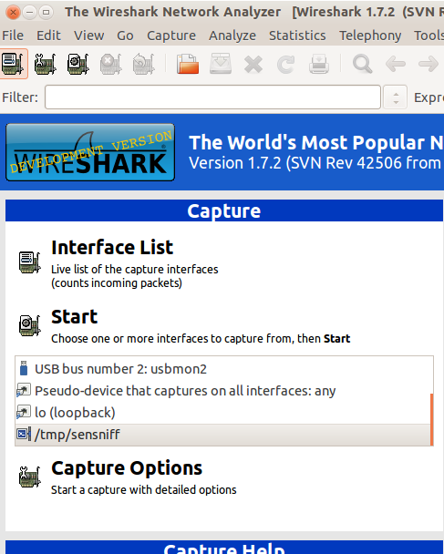
When you open Wireshark, there’s a couple of toolbars at the top, an area called Filter, and a few boxes below in the main window. Online directly links you to Wiresharks site, a handy user guide, and information on the security of Wireshark. Under Files, you’ll find Open, which lets you open previously saved captures, and Sample Captures. You can download any of the sample captures through this website, and study the data. This will help you understand what kind of packets Wireshark can capture.
Lastly is the Capture section. This will let you choose your Interface. You can see each of the interfaces that are available. It’ll also show you which ones are active. Clicking details will show you some pretty generic information about that interface.
Under Start, you can choose one or more interfaces to check out. Capture Options allows you to customize what information you see during a capture. Take a look at your Capture Options – under here you can choose a filter, a capture file, and more. Under Capture Help, you can read up on how to capture, and you can check info on Network Media about what interfaces work on what platforms.
Let’s select an interface and click Start. To stop a capture, press the red square in the top toolbar. If you want to start a new capture, hit the green triangle which looks like a shark fin next to it. Now that you have got a finished capture, you can click File, and save, open, or merge the capture. You can print it, you can quit the program, and you can export your packet capture in a variety of ways.
Under edit, you can find a certain packet, with the search options, you can copy packets, you can mark (highlight) any specific packet, or all the packets. Another interesting thing you can do under Edit, is resetting the time value. You’ll notice that the time is in seconds incrementing. You can reset it from the packet you’ve clicked on. You can add a comment to a packet, configure profiles and preferences.
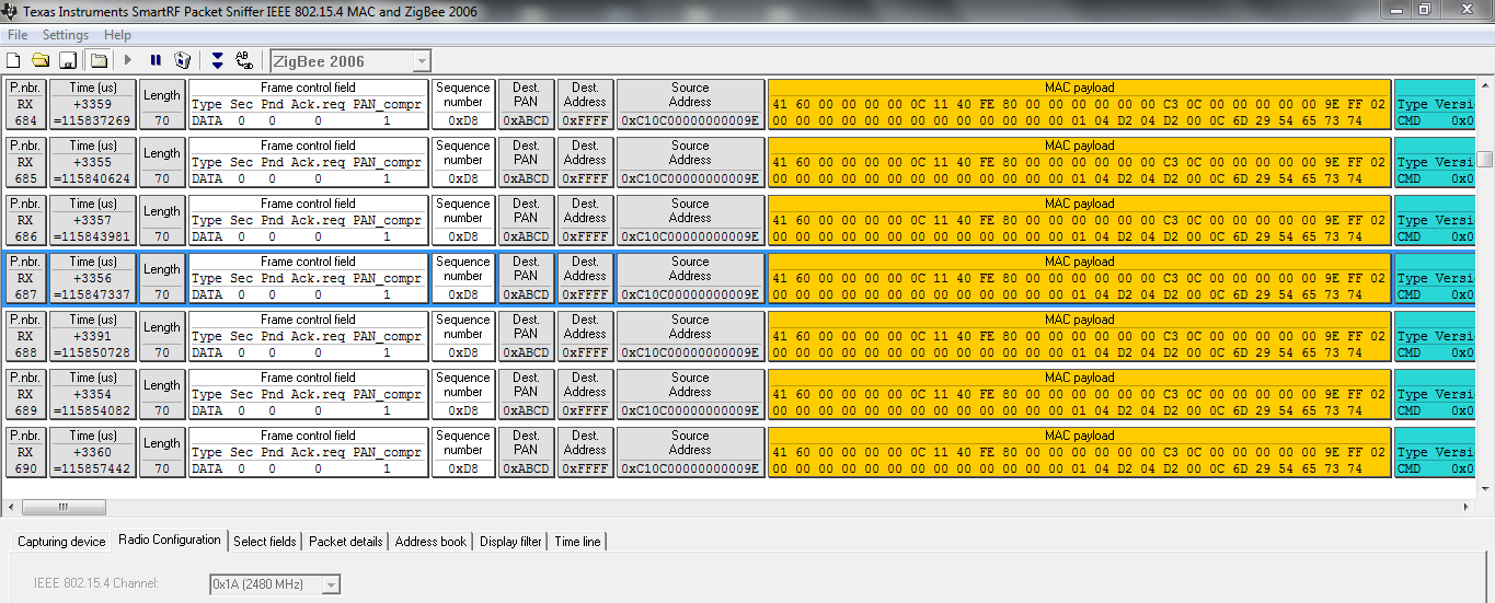
A packet sniffer is a must-have tool for any wireless network application, a sniffer allows to actually see what are you transmitting over the air, verifying both the transmissions are taking place, the frames/packets are properly formatted, and the communication is being done on a given channel.
There are commercial options available, such as the Texas Instruments SmartRF packet Sniffer (http://www.ti.com/tool/packet-sniffer), which can be executed using a CC2531 USB dongle (http://www.ti.com/tool/CC2531EMK) and allows capturing outgoing packets like the one below.
A preferred option is to use the SenSniff application (https://github.com/g-oikonomou/sensniff) paired with a Z1 mote and Wireshark (https://www.wireshark.org), already installed in instant Contiki.
To program the Z1 mote as a packet Sniffer go to the following location:
user@instant-Contiki:~/alignan-Contiki/examples/z1/snifferIn the project-conf.h select the channel to sniff, by changing the RF_CHANNEL and CC2420_CONF_CHANNEL definitions. At the moment of writing this tutorial changing channels from the Sensniff application was not implemented but proposed as a feature, check the Sensniff’s README.md for changes and current status.
Compile and program:
make sniffer.uploadDo not open a login session because the sniffer application uses the serial port to send its findings to the sensniff python script. Open a new terminal, and clone the sensniff project in your home folder:
cd $HOME
git clone https://github.com/g-oikonomou/sensniff
cd sensniff/host
And launch the sensniff application with the following command:
python sensniff.py --non-interactive -d /dev/ttyUSB0 -b 115200Sensniff will read data from the mote over the serial port, dissect the frames and pipe to /tmp/sensniff by default, now we need to connect the other extreme of the pipe to wireshark, else you will get the following warning:
"Remote end not reading"Which is not severe, only means the other pipe endpoint is not connected. You can also save the sniffed frames to open later with wireshark, adding the following argument to the above command -p name.pcap, which will save the session output in a name.pcap file. Change the naming and location in where to store the file accordingly.
Open another terminal and launch wireshark with the following command, which will add the pipe as a capture interface:
sudo wireshark -i /tmp/sensniffSelect the /tmp/sensniff interface from the droplist and click Start just above.
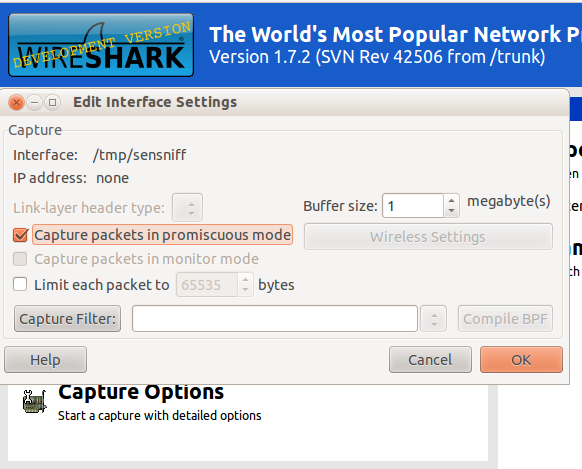
Be sure the pipe is configured to capture packets in promiscuous mode, alternatively you can increase the buffer size, but 1Mb is sufficient enough.
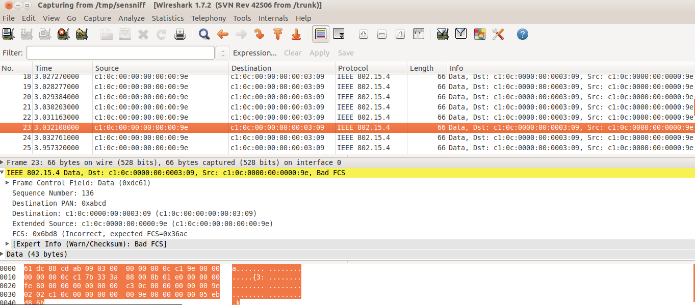
And the captured frames should start to appear on screen.
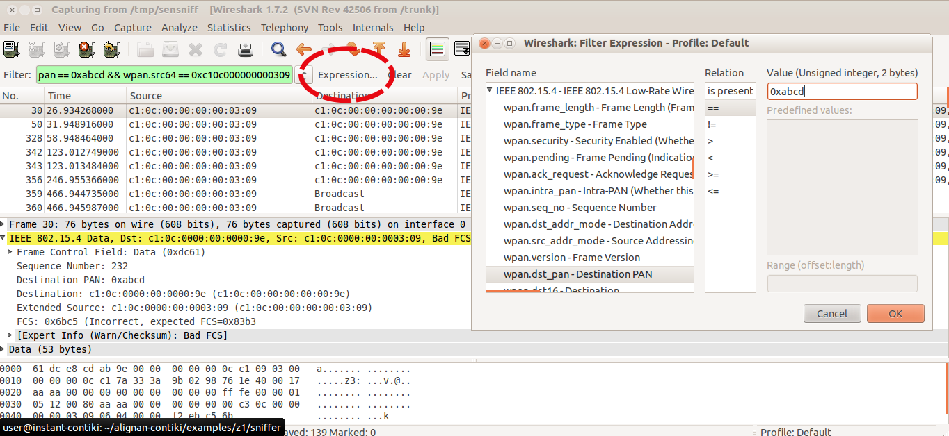
You can add specific filters to limit the frames being shown on screen, for this example make click at the Expression button and a list of available attributes per protocol are listed, scroll down until the IEEE 802.15.4 and check the available filters. You can also chain different filter arguments using the Filter box, in this case we only wanted to check the frames belonging to the PAN 0xABCD and coming from node c1:0c::0309, so we used the wpan.dst_pan and wpan.src64 attributes.
When closing the Sensniff python application, a session information is provided reporting the statistics:
Frame Stats:
         Non-Frame: 6
         Not Piped: 377
    Dumped to PCAP: 8086
             Piped: 7709
Captured: 8086| Excercise: sniff the traffic! try to filter outgoing and incoming data packets using your own custom rules. |
10.2. Foren6
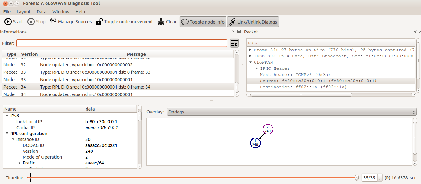
Another must-to-have tool for analyzing and debugging 6loWPAN/IPv6 networks is Foren6 (http://cetic.github.io/foren6/), It uses a passive sniffer devices to reconstruct a visual and textual representation of network information, with a friendly graphical user interface and customizable layout, and allows amongst others to rewind the packet capture history and replay a previous packet trace.

To install follow the instructions at http://cetic.github.io/foren6/install.html
Then to program a Z1 mote as sniffer:
git clone https://github.com/cetic/Contiki
cd Contiki
git checkout sniffer
cd examples/sniffer
make TARGET=z1.upload
Then to connect to Foren6,
MISSING
11. Simple application: UDP Server and client
Normal UDP or TCP transactions require a server-client model, in which the communication is made in sockets, which is an IP address and a port number. What we will do in this example is to forward to the receiver connected to a PC (via USB) temperature sensor data to be published to Ubidots.
| You will need two nodes. The one sending the temperature data is the server, while the one connected to the PC via USB is the client. |
This example relies on a service ID, which allows registering, disseminating, and looking up services. A service is identified by an 8-bit integer between 1 and 255. Integers below 128 are reserved for system services. When setting up the example, we need to decide a service ID for the temperature data. The advantage is that the servers (sending data) don’t need to know the address of the receiver. It is a subscription model where we only need to agree on the service number ID.
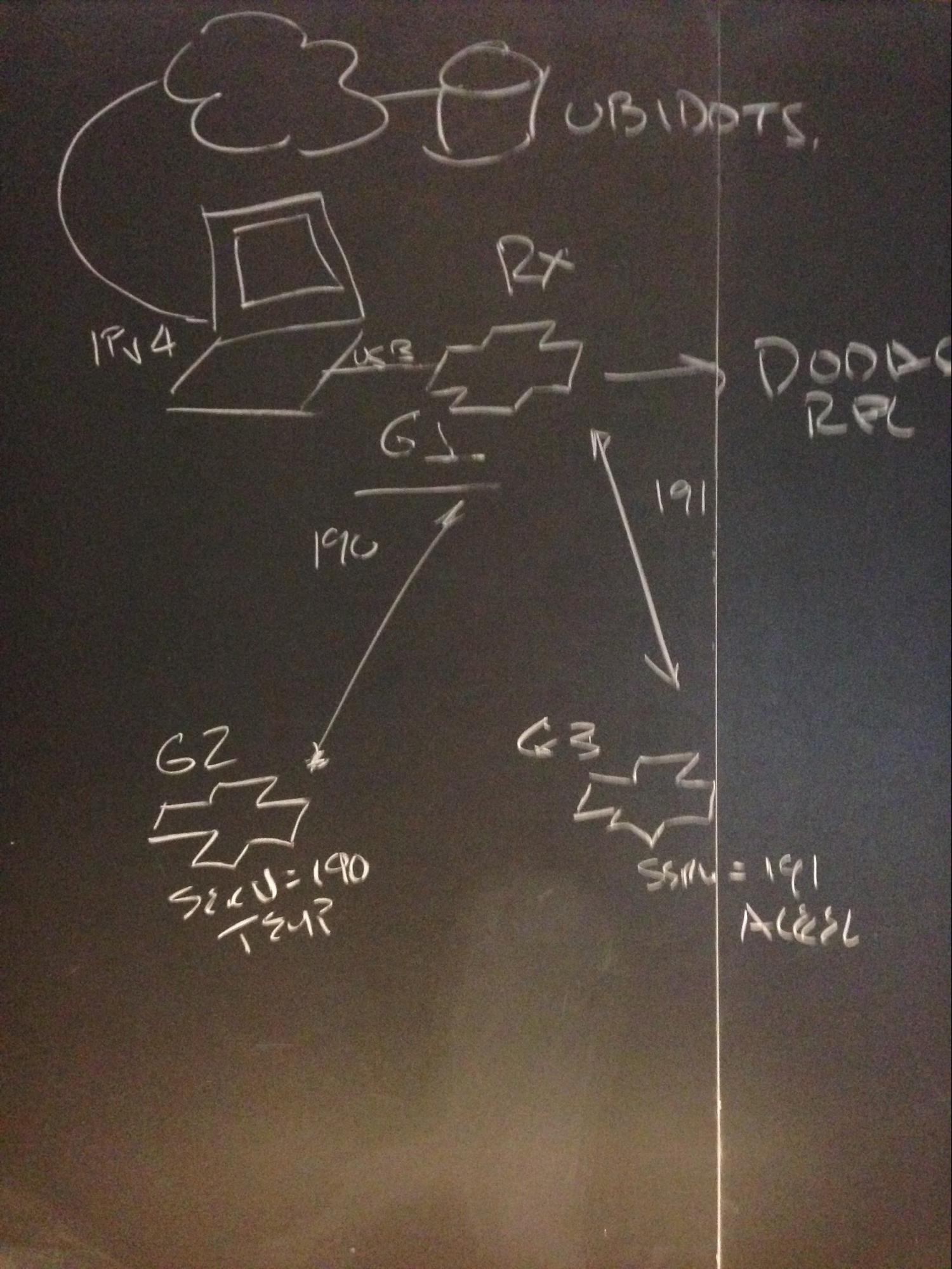
We have three groups. Group 1 hosts the client that received the data from Group 2 and Group 3. Group 2 and 3 are the servers that transmit data. Group 2 sends temperature data and has service ID number 190. Group 3 sends acceleration data and has service ID number 191.
Server side:
Open /home/user/Contiki/examples/ipv6/simple-udp-rpl/unicast-sender.c
At first we are going to add
#include "serial-ubidots.h"
#include "dev/i2cmaster.h"
Group 2:
#include "dev/tmp102.h"
#define SERVICE_ID 190
#define UDP_PORT 1234
Group 3:
#include "dev/adxl345.h"
#define SERVICE_ID 190
#define UDP_PORT 5678
Change the poll rate to something faster:
#define SEND_INTERVAL (15 * CLOCK_SECOND)We have declared a structure at apps/serial-ubidots.h to store the Variable ID and data to be pushed to Ubidots, this will be helpful when sending data wirelessly to the receiver. This is already declared at serial-ubidots.h, do not add this to the example.
struct ubidots_msg_t {
  char var_key[VAR_LEN];
  uint8_t value[2];
};
Declare a structure in our code and a pointer to this structure as below:
static struct ubidots_msg_t msg;
static struct ubidots_msg_t *msgPtr = &msg;
These structures are used to send Ubidots specific information.
In this application we are going to use global IPv6 addresses besides the link-local ones, the function set_global_address initializes our IPv6 address with the prefix aaaa::, and generates also the link local addressing based on the MAC address.
static void
set_global_address(void)
{
  uip_ipaddr_t ipaddr;
  int i;
  uint8_t state;
  // Initialize the IPv6 address as below
  uip_ip6addr(&ipaddr, 0xaaaa, 0, 0, 0, 0, 0, 0, 0);
  // Set the last 64 bits of an IP address based on the MAC address
  uip_ds6_set_addr_iid(&ipaddr, &uip_lladdr);
  // Add to our list addresses
  uip_ds6_addr_add(&ipaddr, 0, ADDR_AUTOCONF);
  printf("IPv6 addresses: ");
  for(i = 0; i < UIP_DS6_ADDR_NB; i++) {
  state = uip_ds6_if.addr_list[i].state;
  if(uip_ds6_if.addr_list[i].isused &&
     (state == ADDR_TENTATIVE || state == ADDR_PREFERRED)) {
    uip_debug_ipaddr_print(&uip_ds6_if.addr_list[i].ipaddr);
    printf("\n");
  }
  }
}
Now inside the PROCESS_THREAD(unicast_sender_process, ev, data), right after the set_global_address() call, we initialize our sensors:
Group 2:
int16_t temp;
tmp102_init();
Group 3:
accm_init();And we pass our variable ID obtained at Ubidots to the ubidots message structure as follows:
memcpy(msg.var_key, "545a202b76254223b5ffa65f", VAR_LEN);
printf("VAR %s\n", msg.var_key);
This function returns the address of the node offering a specific service. If the service is not known, the function returns NULL. If there are more than one nodes offering the service, this function returns the address of the node that most recently announced its service.
addr = servreg_hack_lookup(SERVICE_ID);If we have the receiver node in our services list, then we take a measure from the sensor, pack it into the byte buffer, and send the information to the receiver node by passing the structure as an array using the pointer to the structure, specifying the size in bytes.
The UBIDOTS_MSG_LEN is the sum of the Variable ID string length (24 bytes) plus the sensor reading size (2 bytes).
Replace the existing if (addr != NULL) block with the following:
Group 2:
if (addr != NULL) {

    temp = tmp102_read_temp_x100();
    msg.value[0] = (uint8_t)((temp & 0xFF00) >> 8);
    msg.value[1] = (uint8_t)(temp & 0x00FF);

    printf("Sending temperature reading -> %d via unicast to ", temp);
    uip_debug_ipaddr_print(addr);
    printf("\n");

    simple_udp_sendto(&unicast_connection, msgPtr, UBIDOTS_MSG_LEN, addr);
} else {
    printf("Service %d not found\n", SERVICE_ID);
}
Group 3:
Replace inside the if (addr != NULL) conditional with the following:
msg.value[0] = accm_read_axis(X_AXIS);
msg.value[1] = accm_read_axis(Y_AXIS);
printf("Sending temperature reading -> %d via unicast to ", temp);
uip_debug_ipaddr_print(addr);
printf("\n");
simple_udp_sendto(&unicast_connection, msgPtr, UBIDOTS_MSG_LEN, addr);
And finally add the serial-ubidots app to our Makefile:
APPS = servreg-hack serial-ubidotsIf the address is NULL it can means the receiver node is not present yet.
connecting to /dev/ttyUSB0 (115200) [OK]
Rime started with address 193.12.0.0.0.0.3.9
MAC c1:0c:00:00:00:00:03:09 Ref ID: 255
Contiki-2.6-1796-ga50bc08 started. Node id is set to 377.
CSMA ContikiMAC, channel check rate 8 Hz, radio channel 26
Tentative link-local IPv6 address fe80:0000:0000:0000:c30c:0000:0000:0309
Starting 'Unicast sender example process'
IPv6 addresses: aaaa::c30c:0:0:309
fe80::c30c:0:0:309
VAR 545a202b76254223b5ffa65f
Service 190 not found
Client side:
Open /home/user/Contiki/examples/ipv6/simple-udp-rpl/unicast-receiver.c
Add the Ubidots app:
#include "serial-ubidots.h"Add the services we are interested in, each one to be received in a different UDP port:
#define SERVICE_ID 190
#define UDP_PORT_TEMP  1234
#define UDP_PORT_ACCEL 5678
You can delete the SERVICE_ID, SEND_INTERVAL and SEND_TIME definitions.
RPL is on the IETF standards track for routing in low-power and lossy networks. The protocol is tree-oriented in the sense that one or more root nodes in a network may generate a topology that trickles downward to leaf nodes. In each RPL instance, multiple Directed Acyclic Graphs (DAGs) may exist, each having a different DAG root. A node may join multiple RPL instances, but must only belong to one DAG within each instance.
The receiver creates the RPL DAG and becomes the network root with the same prefix as the servers:
static void
create_rpl_dag(uip_ipaddr_t *ipaddr)
{
  struct uip_ds6_addr *root_if;

  root_if = uip_ds6_addr_lookup(ipaddr);
  if(root_if != NULL) {
  rpl_dag_t *dag;
  uip_ipaddr_t prefix;

  rpl_set_root(RPL_DEFAULT_INSTANCE, ipaddr);
  dag = rpl_get_any_dag();
  uip_ip6addr(&prefix, 0xaaaa, 0, 0, 0, 0, 0, 0, 0);
  rpl_set_prefix(dag, &prefix, 64);
  PRINTF("created a new RPL dag\n");
  } else {
  PRINTF("failed to create a new RPL DAG\n");
  }
}
We now should subscribe to both services (temperature and acceleration), let’s replace the simple_udp_register call inside the PROCESS_THREAD block, after the servreg_hack_register(…) call with the following:
  simple_udp_register(&unicast_connection, UDP_PORT_TEMP,
                    NULL, UDP_PORT_TEMP, receiver);
  simple_udp_register(&unicast_connection, UDP_PORT_ACCEL,
                    NULL, UDP_PORT_ACCEL, receiver);
And at the receiver callback, replace with the following:
static void
receiver(struct simple_udp_connection *c,
       const uip_ipaddr_t *sender_addr,
       uint16_t sender_port,
       const uip_ipaddr_t *receiver_addr,
       uint16_t receiver_port,
       const uint8_t *data,
       uint16_t datalen)
{
  char var_key[VAR_LEN];
  int16_t value;

  printf("Data received from ");
  uip_debug_ipaddr_print(sender_addr);
  printf(" on port %d from port %d\n",
       receiver_port, sender_port);

  if ((receiver_port == UDP_PORT_TEMP) || (receiver_port == UDP_PORT_ACCEL)){

  // Copy the data and send to ubidots, restore missing null termination char
  memcpy(var_key, data, VAR_LEN);
  var_key[VAR_LEN] = "\0";
  value =  data[VAR_LEN] << 8;
  value += data[VAR_LEN + 1];
  printf("Variable -> %s : %d\n", var_key, value);
  send_to_ubidots("fd6c3eb63433221e0a6840633edb21f9ec398d6a", var_key, value);
  }
}
Once the sender and the receivers have started, the following messages are shown on the screen of the receiver:
Starting 'Unicast receiver example process'
IPv6 addresses: aaaa::c30c:0:0:2
fe80::c30c:0:0:2
Data received from aaaa::c30c:0:0:309 on port 1234 from port 1234
Variable -> 545a202b76254223b5ffa65f : 2712

fd6c3eb63433221e0a6840633edb21f9ec398d6a    545b43f776254256ebbef0a6   2712
11.1. IEEE 802.15.4 channels and PAN ID
The IEEE 802.15.4 standard is intended to conform to established radio frequency regulations and defines specific physical (PHY) layers according to country regulations, for example the 2.4-GHz and 868/915-MHz band PHY layers.
The Z1 motes operate on the unlicensed and worldwide available 2.4GHz band, The transmit scheme used is Direct Sequence Spread Spectrum (DSSS) modulation technique, up to 250Kbps data rate, allowing a wireless range of 50-100 mts.
A total of 16 channels are available in the 2.4-GHz band, numbered 11 to 26, each with a bandwidth of 2 MHz and a channel separation of 5 MHz. As other protocols also share this band, such as WiFi IEEE 802.11 and Bluetooth IEEE 802.15, we should be aware of using channels that are not interfered by other devices..
As shown above the channels 15, 20, 25 and 26 are not overlapping WiFi used channels, so typically most IEEE 802.15.4 based devices tend to operate on this frequencies. One handy tool to have is a spectrum analyser to scope the wireless medium, which shows the wireless activity on a given band. A spectrum analyzer will show you the received power at a certain frequency, so you will not know if the power comes from another node, a WiFi device or even a microwave oven! We can use the Z1 mote as a simple spectrum analyser, which sweeps across the list of supported channels and shows its radiated power.
To install the spectrum analyser application to the Z1 mote go to the following directory:
user@instant-Contiki:~/Contiki$ cd examples/z1/rssi_scannerAnd compile, upload and execute the Java application to visualize the radiated power across channels:
make rssi-scanner.upload && make viewrssiThe result are shown below.
You can change the default 26 radio channel in Contiki by changing or redefining the following defines: RF_CHANNEL
But, where are this constants declared? Let’s use a handy command line utility that allows to search for files and content within files, most useful when you need to find a declaration, definition, a file in which an error/warning message is printed, etc. To find where this definition is used by the Z1 platform use this command:
user@instant-Contiki:~/Contiki/platform/z1$ grep -lr "RF_CHANNEL" .Which gives the following result:
./Contiki-conf.hBasically grep as used above uses the following arguments: -lr instructs the utility to search recursively through the directories for the required content between the quotes, from our current location (noted by the dot at the end of the command) transversing the directories structure.
The platform/z1/Contiki-conf.h shows the following information regarding the RF_CHANNEL
#ifdef RF_CHANNEL
#define CC2420_CONF_CHANNEL RF_CHANNEL
#endif

#ifndef CC2420_CONF_CHANNEL
#define CC2420_CONF_CHANNEL          	26
#endif /* CC2420_CONF_CHANNEL */
So we could either change the channel value directly to this file, but this change would affect other applications that perhaps need to operate on a given channel, so we could just override the RF_CHANNEL instead by adding the following to our applications Makefile:
CFLAGS += -DRF_CHANNEL=26Or at compilation time adding the following argument:
DEFINES=RF_CHANNEL=26The PAN ID is an unique Personal Area Network identifier that namely distinguish our network from others in the same channel, thus allowing to subdivide a given channel into sub-networks, each having its own network traffic. By default in Contiki and for the Z1 mote the PAN ID is defined as`0xABCD`.
| Exercise: Search where the PAN_ID is declared (hint: it has the 0xABCD value) and change to something different, then use the Z1 Sniffer and Wireshark to check if the changes were applied. Keep in mind that for 2 devices to talk to each other, the must have the same PAN ID. You can also program the Z1 Sniffer and your test application on a channel other than 26. |
11.2. ETX, LQI, RSSI.
Link Estimation is an integral part of reliable communication in wireless networks. Various link estimation metrics have been proposed to effectively measure the quality of wireless links.
The ETX metric, or expected transmission count, is a measure of the quality of a path between two nodes in a wireless packet data network. ETX is the number of expected transmissions of a packet necessary for it to be received without error at its destination. This number varies from one to infinity. An ETX of one indicates a perfect transmission medium, where an ETX of infinity represents a completely non-functional link. Note that ETX is an expected transmission count for a future event, as opposed to an actual count of a past event. It is hence a real number, and not an integer.
ETX can be used as the routing metric. Routes with a lower metric are preferred. In a route that includes multiple hops, the metric is the sum of the ETX of the individual hops.
LQI (Link Quality Indicator) is a digital value often provide by Chipset vendors, which is an indicator of how well a signal is demodulated, or the strength and quality of the received packet, thus indicating a good or bad wireless medium. The CC2420 radio frequency transceiver used by the Z1 mote typically ranges from 110 (indicates a maximum quality frame) to 50 (typically the lowest quality frames detectable by the transceiver). The example below shows how the Packet Reception Rate decreases as the CC2420 LQI decreases.
RSSI is a generic radio receiver technology metric, used internally in a wireless networking device to determine when the amount of radio energy in the channel is below a certain threshold at which point the medium is clear to transmit. The end-user will likely observe a RSSI value when measuring the signal strength of a wireless network through the use of a wireless network monitoring tool like Wireshark, Kismet or Inssider.
There is no standardized relationship of any particular physical parameter to the RSSI reading, Vendors and chipset makers provide their own accuracy, granularity, and range for the actual power (measured as mW or dBm) and their range of RSSI values (from 0 to RSSI_Max), in the case of the CC2420 radio frequency transceiver on the Z1 mote, the RSSI can range from 0 to -100dBm, values close to 0 are related to good links and values close to -100 are closely related to a bad link, due to multiple factors such as distance, environmental, obstacles, interferences, etc. The image below shows how the Packet Reception Rate (PRR) dramatically decreases as the CC2420 RSSI values are worse.
To print the current channel, RSSI and LQI of the last received packet (thus the link attributes of the link between the node and the sender), we are going to revisit the unicast-receiver.c example, open the file and let’s include the following:
#include "dev/cc2420/cc2420.h"And add the following print statement in the receiver block. The external variables cc2420_last_rssi and cc2420_last_correlation (LQI) are updated on a new incoming packet, so it should match our received packet.
printf("CH: &u RSSI: %d LQI %u\n", cc2420_get_channel(), cc2420_last_rssi, cc2420_last_correlation);We should see something like the following:
Data received from aaaa::c30c:0:0:309 on port 1234 from port 1234
CH: 26 RSSI: -27 LQI 105
Variable -> 545b43f776254256ebbef0a6 : 2650| Exercise: Z1 motes comes in two models: one with an integrated antenna and another with an external antenna. The integrated antenna is a ceramic antenna from Yageo/Phycomp, connected to the CC2420. The external antenna can be connected via a u.FL connector. Try to move away from the receiver and check the received signal on your laptop. What is the max distance? What is the nominal value for 50m with line of sight? Build an application that blinks a green LED when the RSSI is above -55 and a red LED when the RSSI is lower than -55. Does changing the node height and orientation change the RSSI value? If you have one, test the RSSI with an external directional antenna. |
ADD PICTURES
12. Intro to 6LoWPAN
6LoWPAN is a protocol definition to enable IPv6 packets to be carried on top of low power wireless networks. The concept was born from the idea that the Internet Protocol could and should be applied to even the smallest devices. The initial goal was to define an adaptation layer to deal with the requirements imposed by IPv6, such as the increased address sizes and the 1280 byte MTU. The final design takes the concepts used in IPv6 to create a set of headers that allow for the efficient encoding of large IPv6 addresses/headers into a smaller compressed header, while at the same time allowing for the use of various mesh networks and supporting fragmentation and reassembly where needed. The target for IP networking for low-power radio communication are applications that need wireless internet connectivity at lower data rates for devices with very limited form factor. Examples include, but are not limited to: automation and entertainment applications in home, office and factory environments. IPv6 is also in use on the smart grid enabling smart meters and other devices to build a micro mesh network before sending the data back to the billing system using the IPv6 backbone.
The 'Lo' part of 6LoWPAN stands for low-power. The chips used for 6LoWPAN are based on IEEE 802.15.4 radios. These chips require less power so they can run longer on batteries but still have a decent range, although that depends on their frequency. They run at 868 MHz, 900 MHz and 2.4 GHz, depending on the region.
The 'WPAN' is for Wireless Personal Area Network. So this means you can have a network anywhere connected together that consists of sensors or other devices.
The '6' part of 6LoWPAN means that, theoretically, anyone on the Internet can talk to any one of these small 6LoWPAN devices directly because routing would be taken care of through the globe and then to some 'edge router' which would take Ethernet or wifi or whatever else and move it from there to 802.15.4 radio to those small low-power devices.
Some more detailed information about 6LoWPAN is provided below:
Adapting the packet sizes of the two networks. IPv6 requires the maximum transmission unit (MTU) to be at least 1280 Bytes. In contrast, IEEE 802.15.4’s standard packet size is 127 octets. A maximum frame overhead of 25 octets spares 102 octets at the media access control layer. An optional but highly recommended security feature at the link layer poses an additional overhead. For example, 21 octets are consumed for AES-CCM-128 leaving only 81 octets for upper layers.
Address resolution IPv6 nodes are assigned 128 bit IP addresses in a hierarchical manner, through an arbitrary length network prefix. IEEE 802.15.4 devices may use either of IEEE 64 bit extended addresses or, after an association event, 16 bit addresses that are unique within a PAN. There is also a PAN-ID for a group of physically collocated IEEE 802.15.4 devices.
Device and service discovery Since IP-enabled devices may require the formation of ad hoc networks, the current state of neighboring devices and the services hosted by such devices will need to be known. IPv6 neighbour discovery extensions is an internet draft proposed as a contribution in this area.
Security IEEE 802.15.4 nodes can operate in either secure mode or non-secure mode. Two security modes are defined in the specification in order to achieve different security objectives: Access Control List (ACL) and Secure mode.
13. IoT Simulation (Cooja)
Cooja is the Contiki network simulator. Cooja allows large and small networks of Contiki motes to be simulated. Motes can be emulated at the hardware level, which is slower but allows precise inspection of the system behavior, or at a less detailed level, which is faster and allows simulation of larger networks. Cooja is a highly useful tool for Contiki development as it allows developers to test their code and systems long before running it on the target hardware. Developers regularly set up new simulations both to debug their software and to verify the behavior of their systems.
To start Cooja, in the terminal window go to the Cooja directory:
cd contiki/tools/coojaStart Cooja with the command:
ant runWhen Cooja is compiled, it will start with a blue empty window. Now that Cooja is up and running, we can try it out with an example simulation.
13.1. Create a new simulation
Click the File menu and click New simulation. Cooja now opens up the Create new simulation dialog. In this dialog, we may choose to give our simulation a new name, but for this example, we’ll just stick with My simulation. Leave the other options set as default. Click the Create button.
Cooja brings up the new simulation. You can choose what you want to visualize by using the Tools menu. The Network window shows all the motes in the simulated network - it is empty now, since we have no motes in our simulation. The Timeline window shows all communication events in the simulation over time - very handy for understanding what goes on in the network. The Mote output window shows all serial port printouts from all the motes. The Notes window is where we can put notes for our simulation. And the Simulation control window is where we start, pause, and reload our simulation.
13.2. Add motes
Before we can simulate our network, we must add one or more motes. We do this via the Motes menu, where we click on Add motes. Since this is the first mote we add, we must first create a mote type to add. Click Create new mote type and select one of the available mote types. For this example, we click Z1 mote. to create an emulated Z1 mote type. Cooja opens the Create Mote Type dialog, in which we can choose a name for our mote type as well as the Contiki application that our mote type will run. For this example, we stick with the suggested name, and instead click on the Browse button on the right hand side to choose our Contiki application.
13.3. Revisiting broadcast-example in Cooja
Setting up large networks on physical nodes can pose a challenge in terms of instrumenting properly to measure all network elements and having enough equipment available, that’s where Cooja comes handy.
Create a new simulation and define a new Z1 mote-based type of mote called Broadcast, do so by clicking on Motes, Add Motes, Create new mote type and select the Z1 mote. Use the example at examples/ipv6/simple-udp-rpl/broadcast-example.c
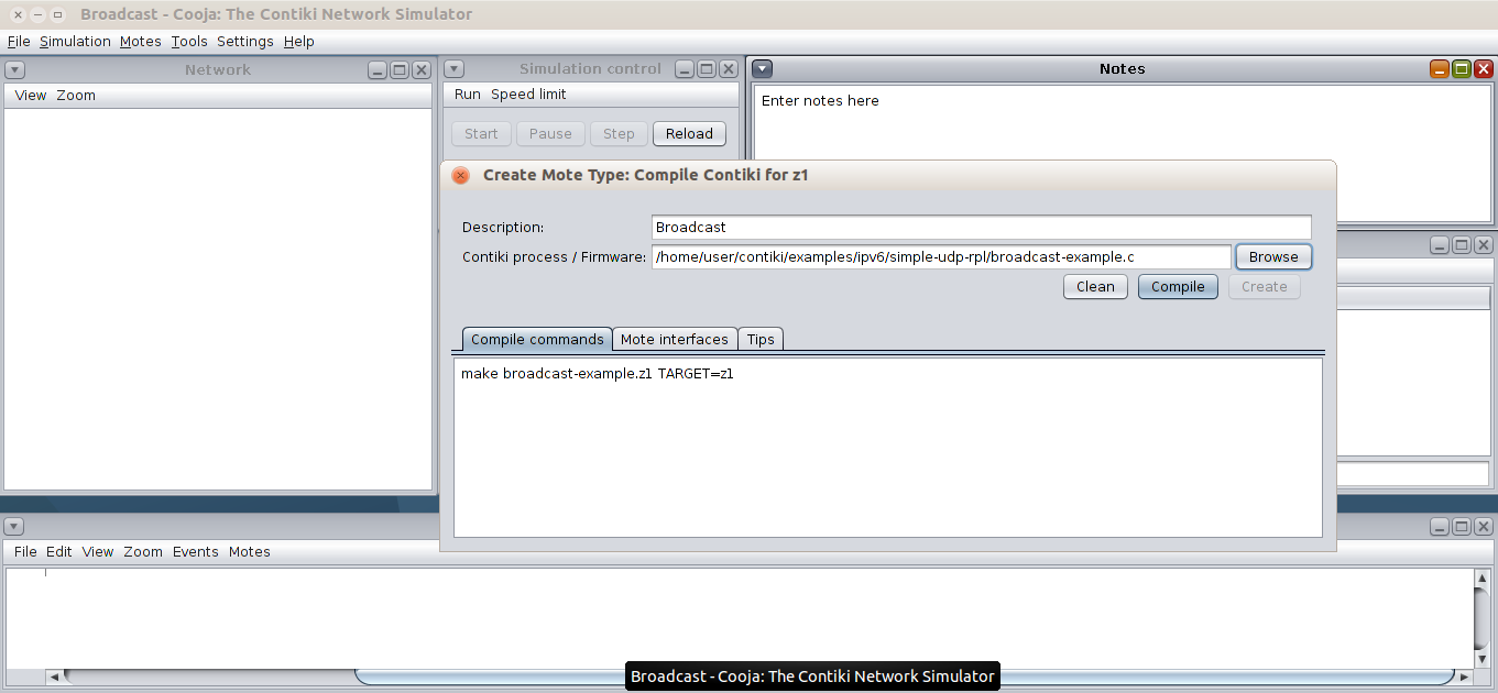
Press Compile and wait for the compilation to end, if there are no errors press Create and it will take you to the next screen. Now add 10 motes using Random positioning. Next in the Network Panel, click on View and add the following: Radio Environment, Mote ID and addresses. Now if you click on a Mote, it will display the Effective Radio coverage (green zone) and interference zone (grey zone) according to the selected medium model.
Be sure to also have the Network, Mote Output and Radio Messages panels in your layout, available at the Tools menu.
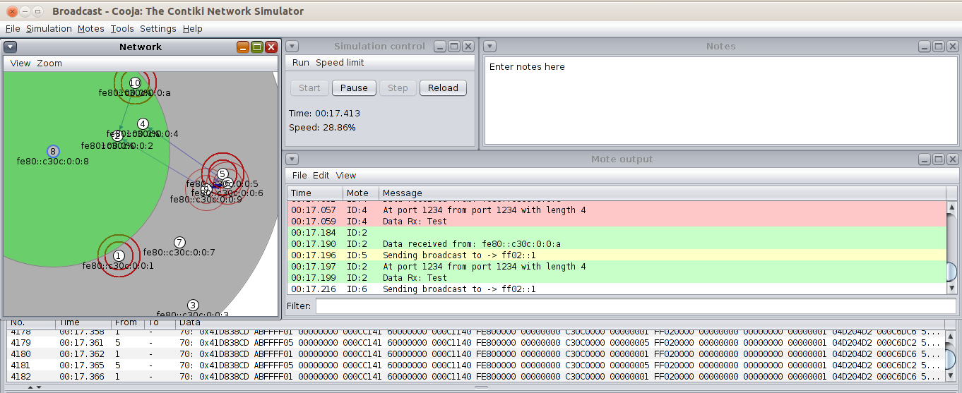
You now should be able to see the network traffic, the messages and the Motes console output, You can pause and start again the simulation to inspect the generated information at your own pace.
HOW CAN I LINK THE SECTION BEFORE TO THIS NEW SECTION?
13.4. Routing Protocol for Low Power Networks (RPL)
RPL is IPv6 routing protocol for low power and lossy networks designed by IETF routing over low power and lossy network (ROLL) group [X], used as the defacto routing protocol in Contiki. RPL is a proactive distance vector protocol, it starts finding the routes as soon as the RPL network is initialized.
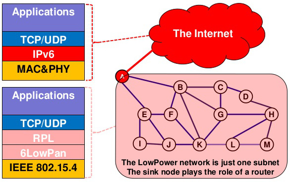
Image source: http://www.slideshare.net/asobimat/rpl-dodag
It supports three traffic patterns: MP2P, point-to-multipoint (P2MP) and point-to-point (P2P).
RPL builds a Destination Oriented DAGs (DODAGs) rooted towards one sink (DAG ROOT) identified by a unique identifier DODAGID. The DODAGs are optimized using a Objective Function (OF) metric identified by an Objective Code Point (OCP), which indicates the dynamic constraints and the metrics such as hop count, latency, expected transmission count, parents selection, energy, etc. A rank number is assigned to each node which can be used to determine its relative position and distance to the root in the DODAG.
Within a given network, there may be multiple, logically independent RPL instances. A RPL node may belong to multiple RPL instances, and may act as a router in some and as a leaf in others. A set of multiple DODAGs can be in a RPL INSTANCE and a node can be a member of multiple RPL INSTANCEs, but can belong to at most one DODAG per DAG INSTANCE.
A trickle timer mechanism [X] regulates DODAG Information Object (DIO) message transmissions, which are used to build and maintain upwards routes of the DODAG, advertising its RPL instance, DODAG ID, RANK and DODAG version number.
A node can request DODAG information by sending DODAG Information Solicitation messages (DIS), soliciting DIO messages from its neighborhoods to update its routing information and join an instance.
Nodes have to monitor DIO messages before joining a DODAG, and then join a DODAG by selecting a parent Node from its neighbors using its advertised latency, OF and RANK. Destination Advertisement Object (DAO) messages are used to maintain downward routes by selecting the preferred parent with lower rank and sending a packet to the DAG ROOT through each of the intermediate Nodes.
PLACE IMAGE SHOWING RPL MESSAGES HERE !!!
RPL has two mechanisms to repair the topology of the DODAG, one to to avoid looping and allow nodes to join/rejoin, and other called global repair [X]. Global repair is initiated at the DODAG ROOT by incrementing the DODAG Version Number to create a new DODAG Version.
Exercise: Go to core/net/rpl and navigate through the C files, look for DEBUG defines and change its value to DEBUG_PRINT, this will print out to screen useful information allowing to better understand the RPL mechanics.
|
14. Connecting our network to the world
We now want to go entirely IPv6, so that our nodes can be reached by the Internet!
We expect your machine to have an IPv6 address, either via the existing cabled network or via a tunnel (such as Gogo6 or Hurricane Electric or others).
In the past examples we have deployed and analyzed link-local networks only, now we will take a step further and connect our networks to external ones, allowing them to be reachable from outside and communicate globally to other networks using 6loWPAN and IPv6.
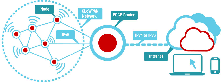
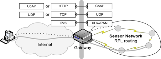
14.1. The border router
The border router or edge router is typically a device sitting at the edge of our network which allow us to talk to outside networks, using its built-in network interfaces, such as WiFI, Ethernet, Serial, etc. In Contiki the current and most used border router application implements a serial-based interface called SLIP, it allows to connect a given mote to a host using scripts like tunslip6 (tools/tunslip6) over the serial port, creating a tunneled network interface, which can be given an IPv6 prefix to set the network global IPv6 addresses.
The most used border router application in Contiki is located at examples/ipv6/rpl-border-router. Motes running the border router application will typically send over the serial port a character sequence, to synchronize with the host over the tunslip6 script. Normally is preferable to configure the border router as a non-sleeping device, so the radio receiver is always on. You can configure the border router settings using the project-conf.h file.
#undef NETSTACK_CONF_RDC
#define NETSTACK_CONF_RDC 	nullrdc_driver
By default the border-router applications includes a built-in web server, displaying information about the network, such as the immediate neighbors (1-hop located) and the known routes to nodes in its network. To enable the web server, the WITH_WEBSERVER flag should be enabled, and by default it will add the httpd-simple.c application.
To compile and upload the border router to the Mote just type:
make TARGET=z1 border-router.uploadAnd to connect the border router to your host run:
make make TARGET=z1 connect-routerBy default it will try to connect to a mote at port /dev/ttyUSB0 using the following serial settings: 115200 baudrate 8N1. If you do not specify an IPv6 prefix it will use the default aaaa::1/64, to specify a specific one run the tunslip tool instead using the following:
make make TARGET=z1 connect-router PREFIX=2001:abcd:dead:beef::1/64You can also compile and run the tunslip6 tool directly from the tools location, to compile just type:
cc tunslip6.c -o tunslip6And to run with specific arguments, if you are required to use a Z1 mote connected to a specific serial port, or require to name your tunnel connection with a specific naming, or proxify to a given address and port. Run ./tunslip -H for more information.
The next example is going to be executed using Cooja, the main objective behind is to deploy a multi-hop network, reachable world-wide using IPv6, effectively connecting our simulation to real-word devices.Open Cooja and load the file at examples/z1/ipv6/z1-websense/example-z1-websense.csc.
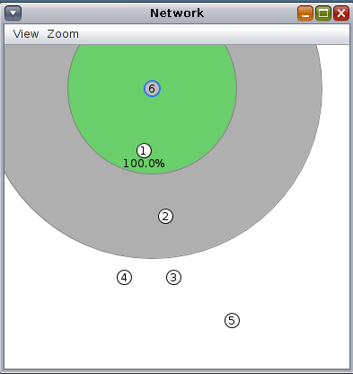
The first noticeable thing about the example is the topology at the Network panel, the Node 6 corresponds to the Border Router Mote, which has only 1 neighbor in its wireless coverage area, and downwards we can see the Border Router being 4-hops apart from the Mote 5. The example contain a step-by-step guide in the Notes panel for you to also follow.
Motes 1 to 5 have been programed with an example called z1-websense, which is a small built-in webserver displaying a history chart with the battery and temperature readings of the Mote, accessible from our web browsers.
Now enable the Border Router (from now on BR) to connect over the serial socket to our host, right-click the BR and select the Serial Socket (SERVER) option from the More tools panel. This will allow us to connect to the simulated BR via the tunslip6 script, run the tool by typing:
sudo ./tunslip6 -a 127.0.0.1 -p 60001 aaaa::1/64Or from the examples/ipv6/rpl-border-router location you can run instead:
make connect-router-coojaYou can replace the IPv6 prefix with your own, the output is shown below. The connection status is shown in the Serial Socket panel in your Cooja layout, it should have changed from listening to Connected.
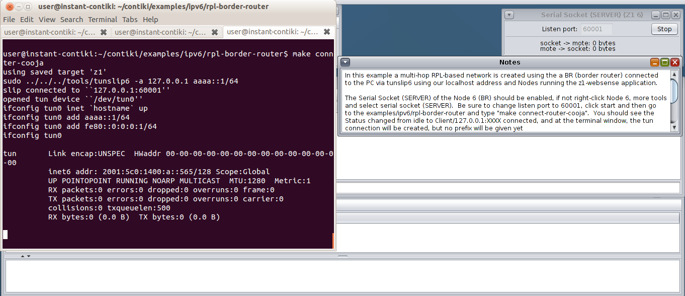
Notice the tunnel connection has been created but no prefix has been given yet. At the Simulation control panel click Start, we should see the BR receiving the aaaa:: prefix by default, thus creating the global server IPv6 address, and it will start sending DIO messages to advertise itself, the Nodes 1-5 will send multicast DIS to request DAG information.
Finally Node 1 (in range of BR) will receive the BR DIO, add BR as preferred parent, joining the newly found instance, replying to BR with a DAO to advertise itself to the BR. Node 1 will multicast DIO messages, Node 2 will receive it, join the instance through Node 1, and reply with a DAO message, which will be used by Node 1 to add Node 2 to its routing table, then forward it upstream to BR.
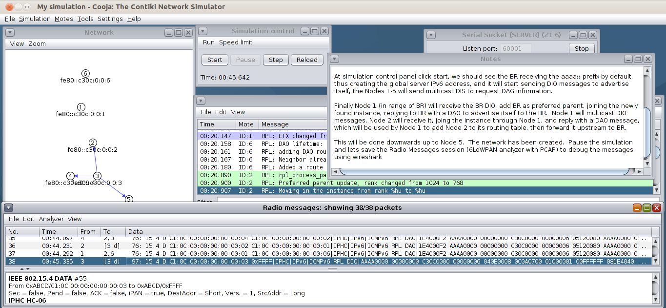
You can pause the simulation and examine the packets and console output at your own pace, simply click the Pause button at the Simulation Control panel. When you are done click Restart. To check we have connectivity from our host to the simulated Motes, open a terminal console and try to ping the devices like follows:
ping6 aaaa::c30c:0:0:5Replace the prefix with your own.
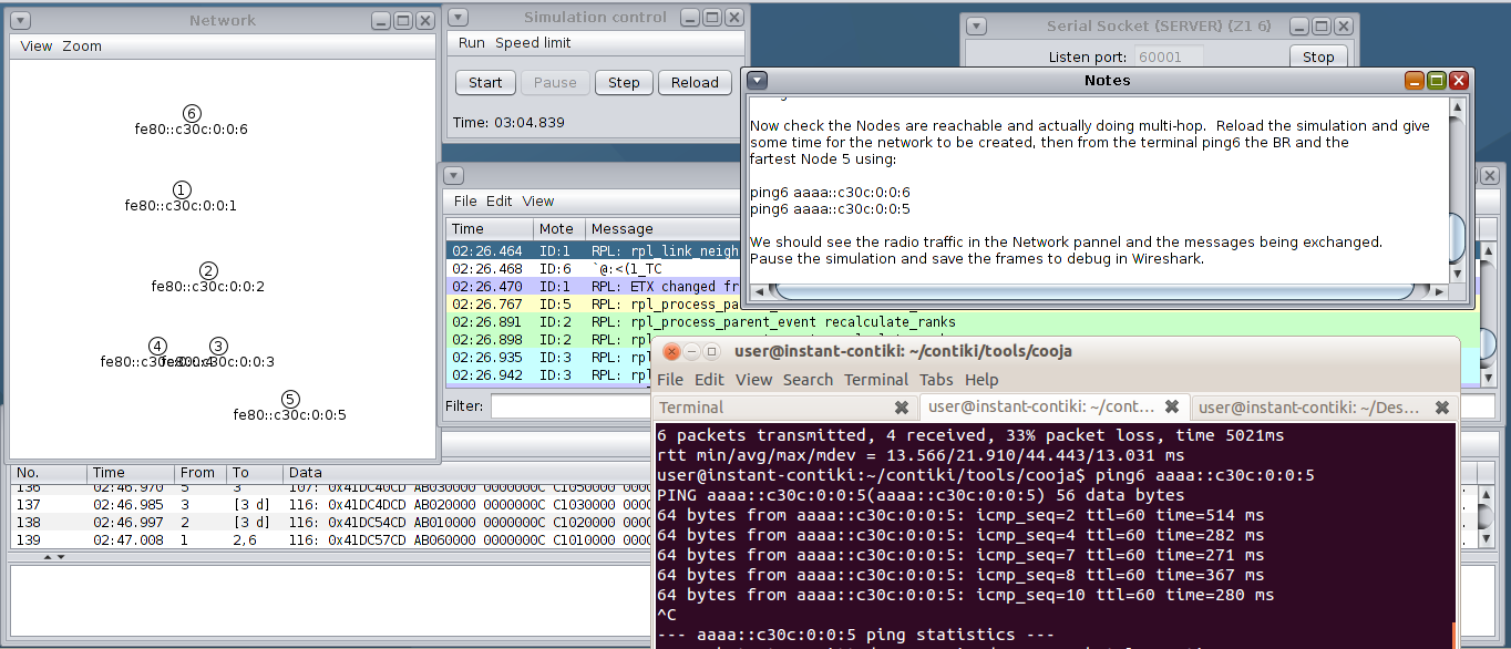
Now open a web browser (Firefox in our example) and type in the URL panel the BR IPv6 public address as follows:
http://[aaaa::c30c:0:0:6]It will display the BR built-in webserver, showing the immediate neighbors and the known routes to the Motes in its instance. We can notice the next-hop neighbor to reach Motes 2 to 5 is Mote 1 as expected.
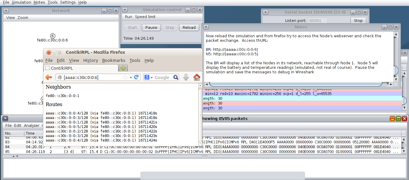
Now to access the webserver running on the nodes, type the global address of any of the Motes in the network. The battery and temperature reading diplayed are emulated values.
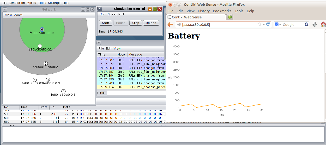
You can examine the packets being sent and received by going through the Radio Messages panel, click on the Analyzer menu and select the 6LoWPAN analyzer with PCAP to format the messages with PCAP to open later using wireshark, click on the File menu and Save To File.
Exercise: connect your simulation
14.2. Setting up IPv6 using gogo6.
In networking, a tunnelling protocol enables new networking functions while still preserving the underlying network as it is. IPv6 tunneling enables IPv6 hosts and routers to connect with other IPv6 hosts and routers over the existing IPv4 Internet. The main purpose of IPv6 tunneling is to deploy IPv6 as well as maintain compatibility with the existing base of IPv4 hosts and routers. IPv6 tunneling encapsulates IPv6 datagrams within IPv4 packets. The encapsulated packets travel across an IPv4 Internet until they reach their destination host or router. The IPv6-aware host or router decapsulates the IPv6 datagrams, forwarding them as needed.
Several tunnel brokers have been developed along with a Tunnel Setup Protocol (TSP). TSP allows IPv4 or IPv6 packets to be encapsulated and carried over IPv4, IPv6 or IPv4 NATs. TSP sets up the tunnel parameters between a user and a server. It handles authentication, encapsulation, IP address assignment and DNS functionality.
One of these TSP providers is gogo6, which provides the gogoCLIENT. The gogoCLIENT connected to the Freenet6 service provides IPv6 connectivity so you can test your v6 network, service or app.
To use the free gogo6 service, setup an account at http://www.gogo6.com/profile/gogoCLIENT
To set up the client on Ubuntu, first install the client with:
sudo apt-get install gogocModify the config file from /etc/gogoc/gogoc.conf with
sudo nano -w /etc/gogoc/gogoc.conf.Locate and modify the following lines:
userid= your_freenet6_id
passwd= your_password
server= broker.freenet6.net
Start the gogo client with
sudo /etc/init.d/gogoc startand you are ready to go.
Try a ping to ipv6.google.com with
ping6 ipv6.google.comIf you can ping google via IPv6, you are ready to go!
You can use http://lg.as6453.net/bin/lg.cgi to check if your machine is visible from the Internet
15. What is REST?
REST stands for Representational State Transfer. (It is sometimes spelled "ReST".) It relies on a stateless, client-server, cacheable communications protocol - and in virtually all cases, the HTTP protocol is used.
REST and the Internet of Things (and Services) can be an excellent match. REST implementations are lightweight: HTTP clients and servers are now available even on the smallest, IP-enabled platforms.
The key abstraction of a RESTful web service is the resource, not a service. Sensors, actors and control systems in general can be elegantly represented as resources and their service exposed through a RESTful web service.
RESTful applications use HTTP requests to post data (create and/or update), read data (e.g., make queries), and delete data. Thus, REST uses HTTP for all four CRUD (Create/Read/Update/Delete) operations.
Despite being simple, REST is fully-featured; there’s basically nothing you can do in Web Services that can’t be done with a RESTful architecture. REST is not a standard.
16. What is COAP?
Constrained Application Protocol (CoAP) is a software protocol intended to be used in very simple electronics devices that allows them to communicate interactively over the Internet. It is particularly targeted for small low power sensors, switches, valves and similar components that need to be controlled or supervised remotely, through standard Internet networks. CoAP is an application layer protocol that is intended for use in resource-constrained internet devices, such as WSN nodes. CoAP is designed to easily translate to HTTP for simplified integration with the web, while also meeting specialized requirements such as multicast support, very low overhead, and simplicity. Multicast, low overhead, and simplicity are extremely important for Internet of Things (IoT) and Machine-to-Machine (M2M) devices, which tend to be deeply embedded and have much less memory and power supply than traditional internet devices have. Therefore, efficiency is very important. CoAP can run on most devices that support UDP. CoAP makes use of two message types, requests and responses, using a simple binary base header format. The base header may be followed by options in an optimized Type-Length-Value format. CoAP is by default bound to UDP and optionally to DTLS, providing a high level of communications security.
Any bytes after the headers in the packet are considered the message body if any. The length of the message body is implied by the datagram length. When bound to UDP the entire message MUST fit within a single datagram. When used with 6LoWPAN as defined in RFC 4944, messages should fit into a single IEEE 802.15.4 frame to minimize fragmentation.